Vue lecture

Il y a de nouveaux articles disponibles, cliquez pour rafraîchir la page.
🔲 ☆

When Exactly Will the Eclipse Happen? A Multimillennium Tale of Computation

When Exactly Will the Eclipse Happen? A Multimillennium Tale of Computation

Updated and expanded from a post for the eclipse of August 21, 2017.

IWhen Exactly Will the Eclipse Happen? A Multimillennium Tale of Computation

Preparing for April 8, 2024

On April 8, 2024, there’s going to be a total eclipse of the Sun visible on a line across the US. But when exactly will the eclipse occur at a given location? Being able to predict astronomical events has historically been one of the great triumphs of exact science. But how well can it actually be done now?

The answer is well enough that even though the edge of totality moves at just over 1000 miles per hour, it’s possible to predict when it will arrive at a given location to within perhaps a second. And as a demonstration of this, for the total eclipse back in 2017 we created a website to let anyone enter their geo location (or address) and then immediately compute when the eclipse would reach them—as well as generate many pages of other information.

Click to enlarge

It’s an Old Business

These days it’s easy to find out when the next solar eclipse will be; indeed built right into the Wolfram Language there’s just a function that tells you (in this form the output is the “time of greatest eclipse”):

It’s also easy to find out, and plot, where the region of totality will be:

Or to determine that the whole area of totality (including lots of ocean and some of Canada) will be about a third of the area of the US:

But computing eclipses is not exactly a new business. In fact, the Antikythera device from 2000 years ago even tried to do it—using 37 metal gears to approximate the motion of the Sun and Moon (yes, with the Earth at the center). To me there’s something unsettling—and cautionary—about the fact that the Antikythera device stands as such a solitary piece of technology, forgotten but not surpassed for more than 1600 years.

But right there on the bottom of the device there’s an arm that moves around, and when it points to an Η or Σ marking, it indicates a possible Sun or Moon eclipse. The way of setting dates on the device is a bit funky (after all, the modern calendar wouldn’t be invented for another 1500 years), but if one takes the simulation on the Wolfram Demonstrations Project (which was calibrated back in 2012 when the Demonstration was created), and turns the crank to set the device for April 8, 2024, here’s what one gets:

Click to enlarge

Antikythera device in action

And, yes, all those gears move so as to line the Moon indicator up with the Sun—and to make the arm on the bottom point right at an H—just as it should for a solar eclipse. It’s amazing to see this computation successfully happen on a device designed 2000 years ago.

Of course the results are a lot more accurate today. Though, strangely, despite all the theoretical science that’s been done, the way we actually compute the position of the Sun and Moon is conceptually very much like the gears—and effectively epicycles—of the Antikythera device. It’s just that now we have the digital equivalent of hundreds of thousands of gears.

Why Do Eclipses Happen?

A total solar eclipse occurs when the Moon gets in front of the Sun from the point of view of a particular location on the Earth. And it so happens that at this point in the Earth’s history the Moon can just block the Sun because it has almost exactly the same angular diameter in the sky as the Sun (about 0.5° or 30 arc-minutes).

So when does the Moon get between the Sun and the Earth? Well, basically every time there’s a new moon (i.e. once every lunar month). But we know there isn’t an eclipse every month. So how come?

Well, actually, in the analogous situation of Ganymede and Jupiter, there is an eclipse every time Ganymede goes around Jupiter (which happens to be about once per week). Like the Earth, Jupiter’s orbit around the Sun lies in a particular plane (the “plane of the ecliptic”). And it turns out that Ganymede’s orbit around Jupiter also lies in essentially the same plane. So every time Ganymede reaches the “new moon” position (or, in official astronomy parlance, when it’s aligned “in syzygy”—pronounced sizz-ee-gee), it’s in the right place to cast its shadow onto Jupiter, and to eclipse the Sun wherever that shadow lands. (From Jupiter, Ganymede appears about 3 times the size of the Sun.)

But our Moon is different. Its orbit doesn’t lie in the plane of the ecliptic. Instead, it’s inclined at about 5°. (How it got that way is unknown, but it’s presumably related to how the Moon was formed.) But that 5° is what makes eclipses so comparatively rare: they can only happen when there’s a “new moon configuration” (syzygy) right at a time when the Moon’s orbit passes through the plane of the ecliptic.

To show what’s going on, let’s draw an exaggerated version of everything. Here’s the Moon going around the Earth, colored red whenever it’s close to the plane of the ecliptic:

Now let’s look at what happens over the course of about a year. We’re showing a dot for where the Moon is each day. And the dot is redder if the Moon is closer to the plane of the ecliptic that day. (Note that if this was drawn to scale, you’d barely be able to see the Moon’s orbit, and it wouldn’t ever seem to go backwards like it does here.)

Now we can start to see how eclipses work. The basic point is that there’s a solar eclipse whenever the Moon is both positioned between the Earth and the Sun, and it’s in the plane of the ecliptic. In the picture, those two conditions correspond to the Moon being as far as possible towards the center, and as red as possible. So far we’re only showing the position of the (exaggerated) Moon once per day. But to make things clearer, let’s show it four times a day—and now prune out cases where the Moon isn’t at least roughly lined up with the Sun:

And now we can see that at least in this particular case, there are two points (indicated by arrows) where the Moon is lined up and in the plane of the ecliptic (so shown in red)—and these points will then correspond to solar eclipses.

In different years, the picture will look slightly different, essentially because the Moon is starting at a different place in its orbit at the beginning of the year. Here are schematic pictures for a few successive years:

It’s not so easy to see exactly when eclipses occur here—and it’s also not possible to tell which are total eclipses where the Moon is exactly lined up, and which are only partial eclipses. But there’s at least an indication, for example, that there are “eclipse seasons” in different parts of the year where eclipses happen.

OK, so what does the real data look like? Here’s a plot for 20 years in the past and 20 years in the future, showing the actual days in each year when total and partial solar eclipses occur (the small dots everywhere indicate new moons):

The reason for the “drift” between successive years is just that the lunar month (29.53 days) doesn’t line up with the year, so the Moon doesn’t go through a whole number of orbits in the course of a year, with the result that at the beginning of a new year, the Moon is in a different phase. But as the picture makes clear, there’s quite a lot of regularity in the general times at which eclipses occur—and for example there are usually 2 eclipses in a given year—though there can be more (and in 0.2% of years there can be as many as 5, as there last were in 1935).

To see more detail about eclipses, let’s plot the time differences (in fractional years) between all successive solar eclipses for 100 years in the past and 100 years in the future:

And now let’s plot the same time differences, but just for total solar eclipses:

There’s obviously a fair amount of overall regularity here, but there are also lots of little fine structure and irregularities. And being able to correctly predict all these details has basically taken science the better part of a few thousand years.

Ancient History

It’s hard not to notice an eclipse, and presumably even from the earliest times people did. But were eclipses just reflections—or omens—associated with random goings-on in the heavens, perhaps in some kind of soap opera among the gods? Or were they things that could somehow be predicted?

A few thousand years ago, it wouldn’t have been clear what people like astrologers could conceivably predict. When will the Moon be at a certain place in the sky? Will it rain tomorrow? What will the price of barley be? Who will win a battle? Even now, we’re not sure how predictable all of these are. But the one clear case where prediction and exact science have triumphed is astronomy.

At least as far as the Western tradition is concerned, it all seems to have started in ancient Babylon—where for many hundreds of years, careful observations were made, and, in keeping with the ways of that civilization, detailed records were kept. And even today we still have thousands of daily official diary entries written in what look like tiny chicken scratches preserved on little clay tablets. “Night of the 14th: Cold north wind. Moon was in front of α Leonis. From 15th to 20th river rose 1/2 cubit. Barley was 1 kur 5 siit. 25th, last part of night, moon was 1 cubit 8 fingers behind ε Leonis. 28th, 74° after sunrise, solar eclipse…”

Click to enlarge

If one looks at what happens on a particular day, one probably can’t tell much. But by putting observations together over years or even hundreds of years, it’s possible to see all sorts of repetitions and regularities. And back in Babylonian times the idea arose of using these to construct an ephemeris—a systematic table that said where a particular heavenly body such as the Moon was expected to be at any particular time.

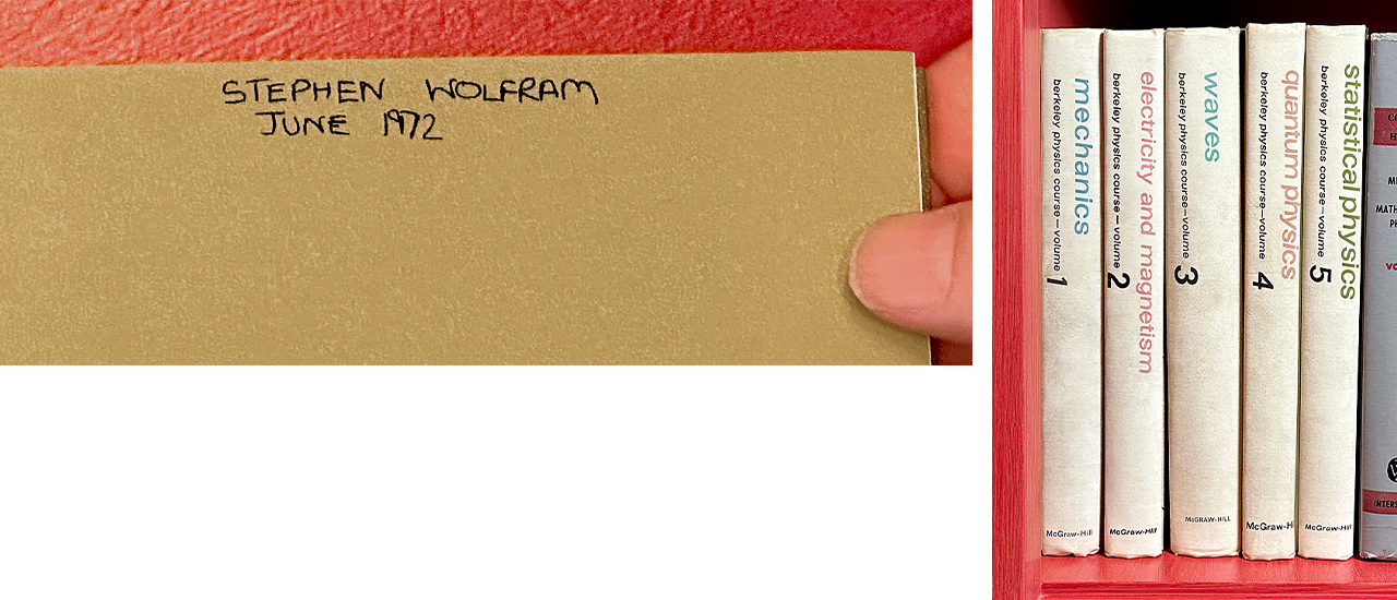
(Needless to say, reconstructing Babylonian astronomy is a complicated exercise in decoding what’s by now basically an alien culture. A key figure in this effort was a certain Otto Neugebauer, who happened to work down the hall from me at the Institute for Advanced Study in Princeton in the early 1980s. I would see him almost every day—a quiet white-haired chap, with a twinkle in his eye—and just sometimes I’d glimpse his huge filing system of index cards which I now realize was at the center of understanding Babylonian astronomy.)

One thing the Babylonians did was to measure surprisingly accurately the repetition period for the phases of the Moon—the so-called synodic month (or “lunation period”) of about 29.53 days. And they noticed that 235 synodic months was very close to 19 years—so that about every 19 years, dates and phases of the Moon repeat their alignment, forming a so-called Metonic cycle (named after Meton of Athens, who described it in 432 BC).

It probably helps that the random constellations in the sky form a good pattern against which to measure the precise position of the Moon (it reminds me of the modern fashion of wearing fractals to make motion capture for movies easier). But the Babylonians noticed all sorts of details of the motion of the Moon. They knew about its “anomaly”: its periodic speeding up and slowing down in the sky (now known to be a consequence of its slightly elliptical orbit). And they measured the average period of this—the so-called anomalistic month—to be about 27.55 days. They also noticed that the Moon went above and below the plane of the ecliptic (now known to be because of the inclination of its orbit)—with an average period (the so-called draconic month) that they measured as about 27.21 days.

And by 400 BC they’d noticed that every so-called saros of about 18 years 11 days all these different periods essentially line up (223 synodic months, 239 anomalistic months and 242 draconic months)—with the result that the Moon ends up at about the same position relative to the Sun. And this means that if there was an eclipse at one saros, then one can make the prediction that there’s going to be an eclipse at the next saros too.

When one’s absolutely precise about it, there are all sorts of effects that prevent precise repetition at each saros. But over timescales of more than 1300 years, there are in fact still strings of eclipses separated from each other by one saros. (Over the course of such a saros series, the locations of the eclipses effectively scan across the Earth; the upcoming eclipse is number 30 in a series of 71 that began in 1501 AD with an eclipse near the North Pole and will end in 2763 AD with an eclipse near the South Pole.)

Any given moment in time will be in the middle of quite a few saros series (right now it’s 40)—and successive eclipses will always come from different series. But knowing about the saros cycle is a great first step in predicting eclipses—and it’s for example what the Antikythera device uses. In a sense, it’s a quintessential piece of science: take many observations, then synthesize a theory from them, or at least a scheme for computation.

It’s not clear what the Babylonians thought about abstract, formal systems. But the Greeks were definitely into them. And by 300 BC Euclid had defined his abstract system for geometry. So when someone like Ptolemy did astronomy, they did it a bit like Euclid—effectively taking things like the saros cycle as axioms, and then proving from them often surprisingly elaborate geometrical theorems, such as that there must be at least two solar eclipses in a given year.

Ptolemy’s Almagest from around 150 AD is an impressive piece of work, containing among many other things some quite elaborate procedures—and explicit tables—for predicting eclipses. (Yes, even in the later printed version, numbers are still represented confusingly by letters, as they always were in ancient Greek.)

Click to enlarge

In Ptolemy’s astronomy, Earth was assumed to be at the center of everything. But in modern terms that just meant he was choosing to use a different coordinate system—which didn’t affect most of the things he wanted to do, like working out the geometry of eclipses. And unlike the mainline Greek philosophers he wasn’t trying to make a fundamental theory of the world; he just wanted whatever epicycles and so on he needed to fit what he observed.

The Dawn of Modern Science

For more than a thousand years Ptolemy’s theory of the Moon defined the state of the art. In the 1300s Ibn al-Shatir revised Ptolemy’s models, achieving somewhat better accuracy. In 1472 Regiomontanus (Johannes Müller), systematizer of trigonometry, published more complete tables as part of his launch of what was essentially the first-ever scientific publishing company. But even in 1543 when Nicolaus Copernicus introduced his Sun-centered model of the solar system, the results he got were basically the same as Ptolemy’s, even though his underlying description of what was going on was quite different.

It’s said that Tycho Brahe got interested in astronomy in 1560 at age 13 when he saw a solar eclipse that had been predicted—and over the next several decades his careful observations uncovered several effects in the motion of the Moon (such as speeding up just before a full moon)—that eventually resulted in perhaps a factor 5 improvement in the prediction of its position. To Tycho eclipses were key tests, and he measured them carefully, and worked hard to be able to predict their timing more accurately than to within a few hours. (He himself never saw a total solar eclipse, only partial ones.)

Click to enlarge

Armed with Tycho’s observations, Johannes Kepler developed his description of orbits as ellipses—introducing concepts like inclination and eccentric anomaly—and in 1627 finally produced his Rudolphine Tables, which got right a lot of things that had been got wrong before, and included all sorts of detailed tables of lunar positions, as well as vastly better predictions for eclipses.

Click to enlarge

Using Kepler’s Rudolphine Tables (and a couple of pages of calculations) the first known actual map of a solar eclipse was published in 1654. And while there are some charming inaccuracies in overall geography, the geometry of the eclipse isn’t too bad.

Whether it was Ptolemy’s epicycles or Kepler’s ellipses, there were plenty of calculations to do in determining the motions of heavenly bodies (and indeed the first known mechanical calculator—excepting the Antikythera device—was developed by a friend of Kepler’s, presumably for the purpose). But there wasn’t really a coherent underlying theory; it was more a matter of describing effects in ways that could be used to make predictions.

So it was a big step forward in 1687 when Isaac Newton published his Principia, and claimed that with his laws for motion and gravity it should be possible—essentially from first principles—to calculate everything about the motion of the Moon. (Charmingly, in his “Theory of the World” section he simply asserts as his Proposition XXII “That all the motions of the Moon… follow from the principles which we have laid down.”)

Newton was proud of the fact that he could explain all sorts of known effects on the basis of his new theory. But when it came to actually calculating the detailed motion of the Moon he had a frustrating time. And even after several years he still couldn’t get the right answer—in later editions of the Principia adding the admission that actually “The apse of the Moon is about twice as swift” (i.e. his answer was wrong by a factor of 2).

Still, in 1702 Newton was happy enough with his results that he allowed them to be published, in the form of a 20-page booklet on the “Theory of the Moon”, which proclaimed that “By this Theory, what by all Astronomers was thought most difficult and almost impossible to be done, the Excellent Mr. Newton hath now effected, viz. to determine the Moon’s Place even in her Quadratures, and all other Parts of her Orbit, besides the Syzygys, so accurately by Calculation, that the Difference between that and her true Place in the Heavens shall scarce be two Minutes…”

Click to enlarge

Newton didn’t explain his methods (and actually it’s still not clear exactly what he did, or how mathematically rigorous it was or wasn’t). But his booklet effectively gave a step-by-step algorithm to compute the position of the Moon. He didn’t claim it worked “at the syzygys” (i.e. when the Sun, Moon and Earth are lined up for an eclipse)—though his advertised error of two arc-minutes was still much smaller than the angular size of the Moon in the sky.

But it wasn’t eclipses that were the focus then; it was a very practical problem of his day: knowing the location of a ship out in the open ocean. It’s possible to determine what latitude you’re at just by measuring how high the Sun gets in the sky. But to determine longitude you have to correct for the rotation of the Earth—and to do that you have to accurately keep track of time. But back in Newton’s day, the clocks that existed simply weren’t accurate enough, especially when they were being tossed around on a ship.

But particularly after various naval accidents, the problem of longitude was deemed important enough that the British government in 1714 established a “Board of Longitude” to offer prizes to help get it solved. One early suggestion was to use the regularity of the moons of Jupiter discovered by Galileo as a way to tell time. But it seemed that a simpler solution (not requiring a powerful telescope) might just be to measure the position of our Moon, say relative to certain fixed stars—and then to back-compute the time from this.

But to do this one had to have an accurate way to predict the motion of the Moon—which is what Newton was trying to provide. In reality, though, it took until the 1760s before tables were produced that were accurate enough to be able to determine time to within a minute (and thus distance to within 15 miles or so). And it so happens that right around the same time a marine chronometer was invented that was directly able to keep good time.

The Three-Body Problem

One of Newton’s great achievements in the Principia was to solve the so-called two-body problem, and to show that with an inverse square law of gravity the orbit of one body around another must always be what Kepler had said: an ellipse.

In a first approximation, one can think of the Moon as just orbiting the Earth in a simple elliptical orbit. But what makes everything difficult is that that’s just an approximation, because in reality there’s also a gravitational pull on the Moon from the Sun. And because of this, the Moon’s orbit is no longer a simple fixed ellipse—and in fact it ends up being much more complicated. There are a few definite effects one can describe and reason about. The ellipse gets stretched when the Earth is closer to the Sun in its own orbit. The orientation of the ellipse precesses like a top as a result of the influence of the Sun. But there’s no way in the end to work out the orbit by pure reasoning—so there’s no choice but to go into the mathematics and start solving the equations of the three-body problem.

In many ways this represented a new situation for science. In the past, one hadn’t ever been able to go far without having to figure out new laws of nature. But here the underlying laws were supposedly known, courtesy of Newton. Yet even given these laws, there was difficult mathematics involved in working out the behavior they implied.

Over the course of the 1700s and 1800s the effort to try to solve the three-body problem and determine the orbit of the Moon was at the center of mathematical physics—and attracted a veritable who’s who of mathematicians and physicists.

An early entrant was Leonhard Euler, who developed methods based on trigonometric series (including much of our current notation for such things), and whose works contain many immediately recognizable formulas:

Click to enlarge

In the mid-1740s there was a brief flap—also involving Euler’s “competitors” Clairaut and d’Alembert—about the possibility that the inverse-square law for gravity might be wrong. But the problem turned out to be with the calculations, and by 1748 Euler was using sums of about 20 trigonometric terms and proudly proclaiming that the tables he’d produced for the three-body problem had predicted the time of a total solar eclipse to within minutes. (Actually, he had said there’d be 5 minutes of totality, whereas in reality there was only 1—but he blamed this error on incorrect coordinates he’d been given for Berlin.)

Mathematical physics moved rapidly over the next few decades, with all sorts of now-famous methods being developed, notably by people like Lagrange. And by the 1770s, for example, Lagrange’s work was looking just like it could have come from a modern calculus book (or from a Wolfram|Alpha step-by-step solution):

Click to enlarge

Particularly in the hands of Laplace there was increasingly obvious success in deriving the observed phenomena of what he called “celestial mechanics” from mathematics—and in establishing the idea that mathematics alone could indeed generate new results in science.

At a practical level, measurements of things like the position of the Moon had always been much more accurate than calculations. But now they were becoming more comparable—driving advances in both. Meanwhile, there was increasing systematization in the production of ephemeris tables. And in 1767 the annual publication began of what was for many years the standard: the British Nautical Almanac.

The almanac quoted the position of the Moon to the arc-second, and systematically achieved at least arc-minute accuracy. The primary use of the almanac was for navigation (and it was what started the convention of using Greenwich as the “prime meridian” for measuring time). But right at the front of each year’s edition were the predicted times of the eclipses for that year—in 1767 just two solar eclipses:

Click to enlarge

The Math Gets More Serious

At a mathematical level, the three-body problem is about solving a system of three ordinary differential equations that give the positions of the three bodies as a function of time. If the positions are represented in standard 3D Cartesian coordinates , the equations can be stated in the form:

3D Cartesian coordinates equations

The {x, y, z} coordinates here aren’t, however, what traditionally show up in astronomy. For example, in describing the position of the Moon one might use longitude and latitude on a sphere around the Earth. Or, given that one knows the Moon has a roughly elliptical orbit, one might instead choose to describe its motions by variables that are based on deviations from such an orbit. In principle it’s just a matter of algebraic manipulation to restate the equations with any given choice of variables. But in practice what comes out is often long and complex—and can lead to formulas that fill many pages.

But, OK, so what are the best kinds of variables to use for the three-body problem? Maybe they should involve relative positions of pairs of bodies. Or relative angles. Or maybe positions in various kinds of rotating coordinate systems. Or maybe quantities that would be constant in a pure two-body problem. Over the course of the 1700s and 1800s many treatises were written exploring different possibilities.

But in essentially all cases the ultimate approach to the three-body problem was the same. Set up the problem with the chosen variables. Identify parameters that, if set to zero, would make the problem collapse to some easy-to-solve form. Then do a series expansion in powers of these parameters, keeping just some number of terms.

The calculations were difficult, and people’s results often didn’t agree. And for example in 1843 Ada Lovelace noted that “In the solution of the famous problem of the Three Bodies, there are, out of about 295 coefficients of lunar perturbations [that had recently been computed]… only 101… agree precisely both in signs and in amount [with previous works]” (going on to say, rather farsightedly, that this was something the Analytical Engine would be able to solve).

By the 1860s Charles Delaunay had, however, spent 20 years developing the most extensive theory of the Moon using series expansions. He’d identified five parameters with respect to which to do his expansions (eccentricities, inclinations, and ratios of orbit sizes)—and in the end he generated about 1800 pages like this (yes, he really needed Mathematica!):

Click to enlarge

But the sad fact was that despite all this effort, he didn’t get terribly good answers. And eventually it became clear why. The basic problem was that Delaunay wanted to represent his results in terms of functions like sin and cos. But in his computations, he often wanted to do series expansions with respect to the frequencies of those functions. Here’s a minimal case:

And here’s the problem. Take a look even at the second term. Yes, the δ parameter may be small. But how about the parameter, standing for time? If you don’t want to make predictions very far out, that’ll stay small. But what if you want to figure out what will happen further in the future?

Well, eventually that term will get big. And higher-order terms will get even bigger. But unless the Moon is going to escape its orbit or something, the final mathematical expressions that represent its position can’t have values that are too big. So in these expressions the so-called secular terms that increase with must somehow cancel out.

But the problem is that at any given order in the series expansion, there’s no guarantee that will happen in a numerically useful way. And in Delaunay’s case—even though with immense effort he often went to 7th order or beyond—it didn’t.

One nice feature of Delaunay’s computation was that it was in a sense entirely algebraic: everything was done symbolically, and only at the very end were actual numerical values of parameters substituted in.

But even before Delaunay, Peter Hansen had taken a different approach—substituting numbers as soon as he could, and dropping terms based on their numerical size rather than their symbolic form. His presentations look less pure (notice things like all those , where is the time in years), and it’s more difficult to tell what’s going on. But as a practical matter, his results were much better, and in fact were used for many national almanacs from about 1862 to 1922, achieving errors as small as 1 or 2 arc-seconds at least over periods of a decade or so. (Over longer periods, the errors could rapidly increase because of the lack of terms that had been dropped as a result of what amounted to numerical accidents.)

Click to enlarge

Both Delaunay and Hansen tried to represent orbits as series of powers and trigonometric functions (so-called Poisson series). But in the 1870s, George Hill in the US Nautical Almanac Office proposed instead using as a basis numerically computed functions that came from solving an equation for two-body motion with a periodic driving force of roughly the kind the Sun exerts on the Moon’s orbit. A large-scale effort was mounted, and starting in 1892 Ernest W. Brown (who had moved to the US, but had been a student of George Darwin, Charles Darwin’s physicist son) took charge of the project and in 1918 produced what would stand for many years as the definitive “Tables of the Motion of the Moon”.

Brown’s tables consist of hundreds of pages like this—ultimately representing the position of the Moon as a combination of about 1400 terms with very precise coefficients:

Click to enlarge

He says right at the beginning that the tables aren’t particularly intended for unique events like eclipses, but then goes ahead and does a “worked example” of computing an eclipse from 381 BC, reported by Ptolemy:

Click to enlarge

It was an impressive indication of how far things had come. But ironically enough the final presentation of Brown’s tables had the same sum-of-trigonometric-functions form that one would get from having lots of epicycles. At some level it’s not surprising, because any function can ultimately be represented by epicycles, just as it can be represented by a Fourier or other series. But it’s a strange quirk of history that such similar forms were used.

Can the Three-Body Problem Be Solved?

It’s all well and good that one can find approximations to the three-body problem, but what about just finding an outright solution—like as a mathematical formula? Even in the 1700s, there’d been some specific solutions found—like Euler’s collinear configuration, and Lagrange’s equilateral triangle. But a century later, no further solutions had been found—and finding a complete solution to the three-body problem was beginning to seem as hopeless as trisecting an angle, solving the quintic, or making a perpetual motion machine. (That sentiment was reflected for example in a letter Charles Babbage wrote Ada Lovelace in 1843 mentioning the “horrible problem [of] the three bodies”—even though this letter was later misinterpreted by Ada’s biographers to be about a romantic triangle, not the three-body problem of celestial mechanics.)

In contrast to the three-body problem, what seemed to make the two-body problem tractable was that its solutions could be completely characterized by “constants of the motion”—quantities that stay constant with time (in this case notably the direction of the axis of the ellipse). So for many years one of the big goals with the three-body problem was to find constants of the motion.

In 1887, though, Heinrich Bruns showed that there couldn’t be any such constants of the motion, at least expressible as algebraic functions of the standard {x, y, z} position and velocity coordinates of the three bodies. Then in the mid-1890s Henri Poincaré showed that actually there couldn’t be any constants of the motion that were expressible as any analytic functions of the positions, velocities and mass ratios.

One reason that was particularly disappointing at the time was that it had been hoped that somehow constants of the motion would be found in n-body problems that would lead to a mathematical proof of the long-term stability of the solar system. And as part of his work, Poincaré also saw something else: that at least in particular cases of the three-body problem, there was arbitrarily sensitive dependence on initial conditions—implying that even tiny errors in measurement could be amplified to arbitrarily large changes in predicted behavior (the classic “chaos theory” phenomenon).

But having discovered that particular solutions to the three-body problem could have this kind of instability, Poincaré took a different approach that would actually be characteristic of much of pure mathematics going forward: he decided to look not at individual solutions, but at the space of all possible solutions. And needless to say, he found that for the three-body problem, this was very complicated—though in his efforts to analyze it he invented the field of topology.

Poincaré’s work all but ended efforts to find complete solutions to the three-body problem. It also seemed to some to explain why the series expansions of Delaunay and others hadn’t worked out—though in 1912 Karl Sundman did show that at least in principle the three-body problem could be solved in terms of an infinite series, albeit one that converges outrageously slowly.

But what does it mean to say that there can’t be a solution to the three-body problem? Galois had shown that there couldn’t be a solution to the generic quintic equation, at least in terms of radicals. But actually it’s still perfectly possible to express the solution in terms of elliptic or hypergeometric functions. So why can’t there be some more sophisticated class of functions that can be used to just “solve the three-body problem”?

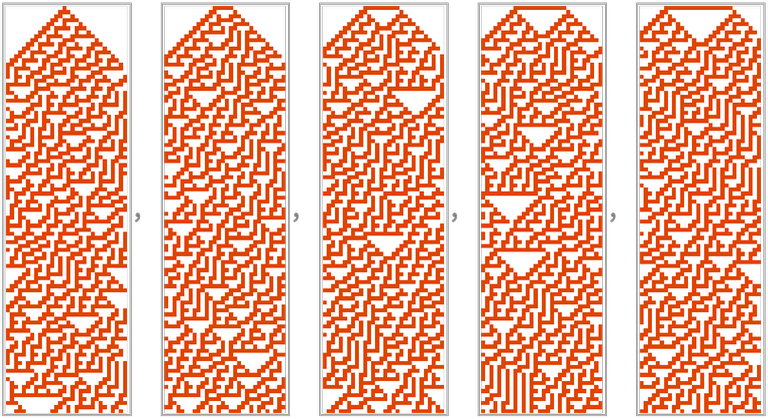
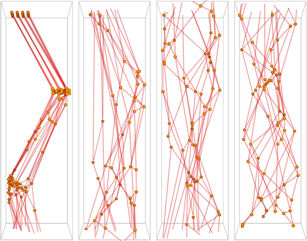
Here are some pictures of what can actually happen in the three-body problem, with various initial conditions:

Click to enlarge

And looking at these immediately gives some indication of why it’s not easy to just “solve the three-body problem”. Yes, there are cases where what happens is fairly simple. But there are also cases where it’s not, and where the trajectories of the three bodies continue to be complicated and tangled for a long time.

So what’s fundamentally going on here? I don’t think traditional mathematics is the place to look. But I think what we’re seeing is actually an example of a general phenomenon I call computational irreducibility that I discovered in the 1980s in studying the computational universe of possible programs.

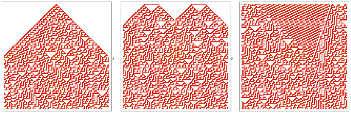
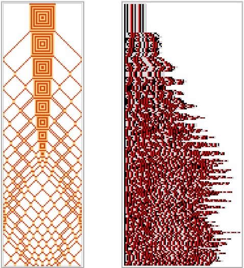
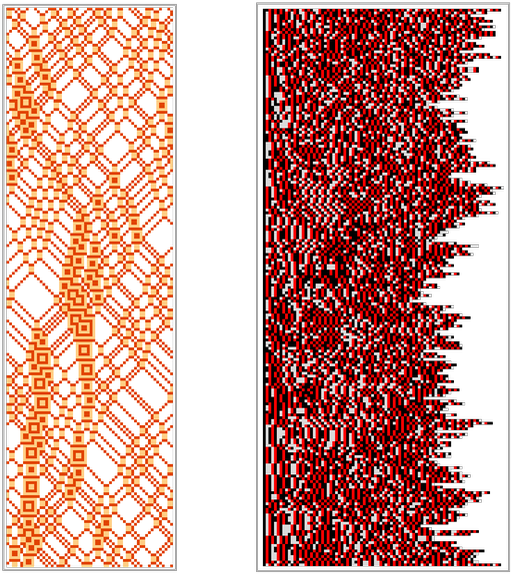
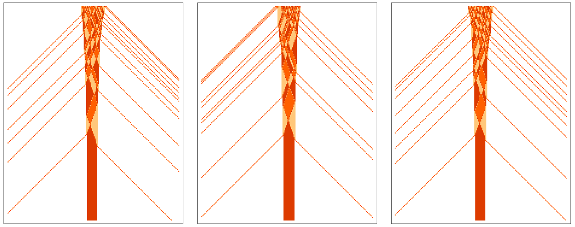
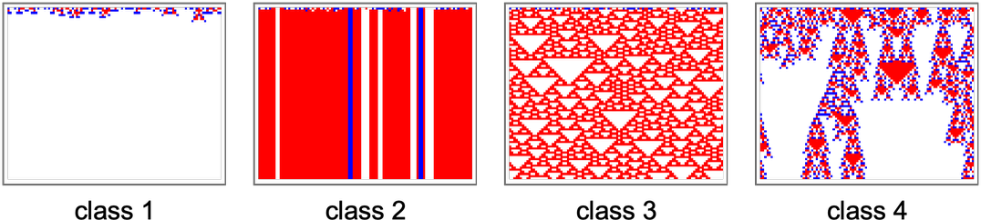
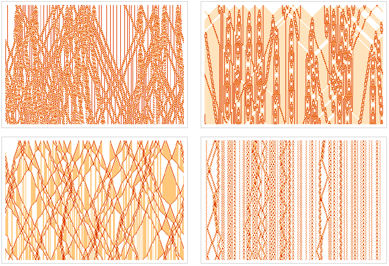
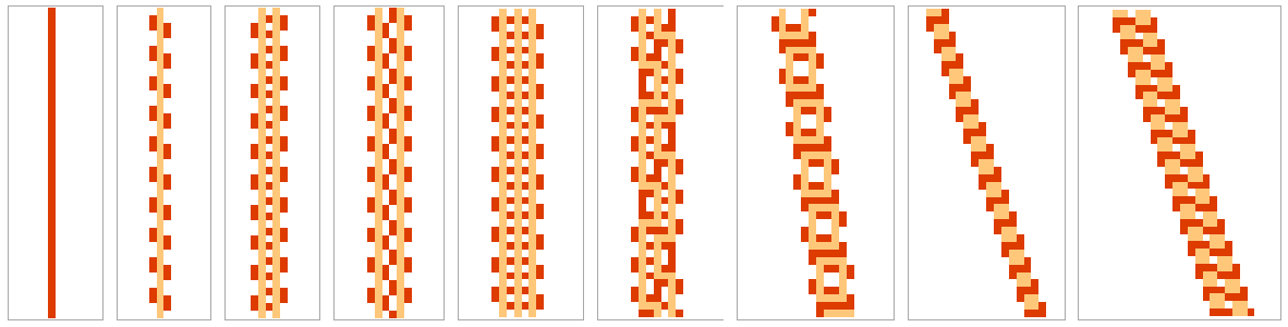
Many programs, like many instances of the three-body problem, behave in quite simple ways. But if you just start looking at all possible simple programs, it doesn’t take long before you start seeing behavior like this:

How can one tell what’s going to happen? Well, one can just keep explicitly running each program and seeing what it does. But the question is: is there some systematic way to jump ahead, and to predict what will happen without tracing through all the steps?

The answer is that in general there isn’t. And what I call the Principle of Computational Equivalence suggests that pretty much whenever one sees complex behavior, there won’t be.

Here’s the way to think about this. The system one’s studying is effectively doing a computation to work out what its behavior will be. So to jump ahead we’d in a sense have to do a more sophisticated computation. But what the Principle of Computational Equivalence says is that actually we can’t—and that whether we’re using our brains or our mathematics or a Turing machine or anything else, we’re always stuck with computations of the same sophistication.

So what about the three-body problem? Well, I strongly suspect that it’s an example of computational irreducibility: that in effect the computations it’s doing are as sophisticated as any computations that we can do, so there’s no way we can ever expect to systematically jump ahead and solve the problem. (We also can’t expect to just define some new finite class of functions that can just be evaluated to give the solution.)

I’m hoping that one day someone will rigorously prove this. There’s some technical difficulty, because the three-body problem is usually formulated in terms of real numbers that immediately have an infinite number of digits—but to compare with ordinary computation one has to require finite processes to set up initial conditions. (Ultimately one wants to show for example that there’s a “compiler” that can go from any program, say for a Turing machine, and can generate instructions to set up initial conditions for a three-body problem so that the evolution of the three-body problem will give the same results as running that program—implying that the three-body problem is capable of universal computation.)

I have to say that I consider Newton in a sense very lucky. It could have been that it wouldn’t have been possible to work out anything interesting from his theory without encountering the kind of difficulties he had with the motion of the Moon—because one would always be running into computational irreducibility. But in fact, there was enough computational reducibility and enough that could be computed easily that one could see that the theory was useful in predicting features of the world (and not getting wrong answers, like with the apse of the Moon)—even if there were some parts that might take two centuries to work out, or never be possible at all.

Newton himself was certainly aware of the potential issue, saying that at least if one was dealing with gravitational interactions between many planets then “to define these motions by exact laws admitting of easy calculation exceeds, if I am not mistaken, the force of any human mind”.
And even today it’s extremely difficult to know what the long-term evolution of the solar system will be.

It’s not particularly that there’s sensitive dependence on initial conditions: we actually have measurements that should be precise enough to determine what will happen for a long time. The problem is that we just have to do the computation—a bit like computing the digits of π—to work out the behavior of the -body problem that is our solar system.

Existing simulations show that for perhaps a few tens of millions of years, nothing too dramatic can happen. But after that we don’t know. Planets could change their order. Maybe they could even collide, or be ejected from the solar system. Computational irreducibility implies that at least after an infinite time it’s actually formally undecidable (in the sense of Gödel’s theorem or the halting problem) what can happen.

One of my children, when they were very young, asked me whether when dinosaurs existed the Earth could have had two moons. For years when I ran into celestial mechanics experts I would ask them that question—and it was notable how difficult they found it. Most now say that at least at the time of the dinosaurs we couldn’t have had an extra moon—though a billion years earlier it’s not clear.

We used to only have one system of planets to study. And the fact that there were (then) 9 of them used to be a classic philosopher’s example of a truth about the world that just happens to be the way it is, and isn’t “necessarily true” (like 2 + 2 = 4). But now of course we know about lots of exoplanets. And it’s beginning to look as if there might be a theory for things like how many planets a solar system is likely to have.

At some level there’s presumably a process like natural selection: some configurations of planets aren’t “fit enough” to be stable—and only those that are survive. In biology it’s traditionally been assumed that natural selection and adaptation is somehow what’s led to the complexity we see. But actually I suspect much of it is instead just a reflection of what generally happens in the computational universe—both in biology and in celestial mechanics. Now in celestial mechanics, we haven’t yet seen in the wild any particularly complex forms (beyond a few complicated gap structures in rings, and tumbling moons and asteroids). But perhaps elsewhere we’ll see things like those obviously tangled solutions to the three-body problem—that come closer to what we’re used to in biology.

It’s remarkable how similar the issues are across so many different fields. For example, the whole idea of using “perturbation theory” and series expansions that has existed since the 1700s in celestial mechanics is now also core to quantum field theory. But just like in celestial mechanics there’s trouble with convergence (maybe one should try renormalization or resummation in celestial mechanics). And in the end one begins to realize that there are phenomena—no doubt like turbulence or the three-body problem—that inevitably involve more sophisticated computations, and that need to be studied not with traditional mathematics of the kind that was so successful for Newton and his followers but with the kind of science that comes from exploring the computational universe.

Approaching Modern Times

But let’s get back to the story of the motion of the Moon. Between Brown’s tables, and Poincaré’s theoretical work, by the beginning of the 1900s the general impression was that whatever could reasonably be computed about the motion of the Moon had been computed.

Occasionally there were tests. Like for example in 1925, when there was a total solar eclipse visible in New York City, and the New York Times perhaps overdramatically said that “scientists [were] tense… [wondering] whether they or Moon is wrong as eclipse lags five seconds behind”. The fact is that a prediction accurate to 5 seconds was remarkably good, and we can’t do all that much better even today. (By the way, the actual article talks extensively about “Professor Brown”—as well as about how the eclipse might “disprove Einstein” and corroborate the existence of “coronium”—but doesn’t elaborate on the supposed prediction error.)

Click to enlarge

As a practical matter, Brown’s tables were not exactly easy to use: to find the position of the Moon from them required lots of mechanical desk calculator work, as well as careful transcription of numbers. And this led Leslie Comrie in 1932 to propose using a punch-card-based IBM Hollerith automatic tabulator—and with the help of Thomas Watson, CEO of IBM, what was probably the first “scientific computing laboratory” was established—to automate computations from Brown’s tables.

Click to enlarge

(When I was in elementary school in England in the late 1960s—before electronic calculators—I always carried around, along with my slide rule, a little book of “4-figure mathematical tables”. I think I found it odd that such a book would have an author—and perhaps for that reason I still remember the name: “L. J. Comrie”.)

By the 1950s, the calculations in Brown’s tables were slowly being rearranged and improved to make them more suitable for computers. But then with John F. Kennedy’s 1962 “We choose to go to the Moon”, there was suddenly urgent interest in getting the most accurate computations of the Moon’s position. As it turned out, though, it was basically just a tweaked version of Brown’s tables, running on a mainframe computer, that did the computations for the Apollo program.

At first, computers were used in celestial mechanics purely for numerical computation. But by the mid-1960s there were also experiments in using them for algebraic computation, and particularly to automate the generation of series expansions. Wallace Eckert at IBM started using FORMAC to redo Brown’s tables, while in Cambridge David Barton and Steve Bourne (later the creator of the “Bourne shell” (sh) in Unix) built their own CAMAL computer algebra system to try extending the kind of thing Delaunay had done. (And by 1970, Delaunay’s 7th-order calculations had been extended to 20th order.)

When I myself started to work on computer algebra in 1976 (primarily for computations in particle physics), I’d certainly heard about CAMAL, but I didn’t know what it had been used for (beyond vaguely “celestial mechanics”). And as a practicing theoretical physicist in the late 1970s, I have to say that the “problem of the Moon” that had been so prominent in the 1700s and 1800s had by then fallen into complete obscurity.

I remember for example in 1984 asking a certain Martin Gutzwiller, who was talking about quantum chaos, what his main interest actually was. And when he said “the problem of the Moon”, I was floored; I didn’t know there still was any problem with the Moon. As it turns out, in writing this post I found out that Gutzwiller was actually the person who took over from Eckert and spent nearly two decades working on trying to improve the computations of the position of the Moon.

Why Not Just Solve It?

Traditional approaches to the three-body problem come very much from a mathematical way of thinking. But modern computational thinking immediately suggests a different approach. Given the differential equations for the three-body problem, why not just directly solve them? And indeed in the Wolfram Language there’s a built-in function NDSolve for numerically solving systems of differential equations.

So what happens if one just feeds in equations for a three-body problem? Well, here are the equations:

Now as an example let’s set the masses to random values:

And let’s define the initial position and velocity for each body to be random as well:

Now we can just use NDSolve to get the solutions (it gives them as implicit approximate numerical functions of ):

And now we can plot them. And now we’ve got a solution to a three-body problem, just like that!

Well, obviously this is using the Wolfram Language and a huge tower of modern technology. But would it have been possible even right from the beginning for people to generate direct numerical solutions to the three-body problem, rather than doing all that algebra? Back in the 1700s, Euler already knew what’s now called Euler’s method for finding approximate numerical solutions to differential equations. So what if he’d just used that method to calculate the motion of the Moon?

The method relies on taking a sequence of discrete steps in time. And if he’d used, say, a step size of a minute, then he’d have had to take 40,000 steps to get results for a month, but he should have been able to successfully reproduce the position of the Moon to about a percent. If he’d tried to extend to 3 months, however, then he would already have had at least a 10% error.

Any numerical scheme for solving differential equations in practice eventually builds up some kind of error—but the more one knows about the equations one’s solving, and their expected solutions, the more one’s able to preprocess and adapt things to minimize the error. NDSolve has enough automatic adaptivity built into it that it’ll do pretty well for a surprisingly long time on a typical three-body problem. (It helps that the Wolfram Language and NDSolve can handle numbers with arbitrary precision, not just machine precision.)

But if one looks, say, at the total energy of the three-body system—which one can prove from the equations should stay constant—then one will typically see an error slowly build up in it. One can avoid this if one effectively does a change of variables in the equations to “factor out” energy. And one can imagine doing a whole hierarchy of algebraic transformations that in a sense give the numerical scheme as much help as possible.

And indeed since at least the 1980s that’s exactly what’s been done in practical work on the three-body problem, and the Earth-Moon-Sun system. So in effect it’s a mixture of the traditional algebraic approach from the 1700s and 1800s, together with modern numerical computation.

The Real Earth-Moon-Sun Problem

OK, so what’s involved in solving the real problem of the Earth-Moon-Sun system? The standard three-body problem gives a remarkably good approximation to the physics of what’s happening. But it’s obviously not the whole story.

For a start, the Earth isn’t the only planet in the solar system. And if one’s trying to get sufficiently accurate answers, one’s going to have to take into account the gravitational effect of other planets. The most important is Jupiter, and its typical effect on the orbit of the Moon is at about the level—sufficiently large that for example Brown had to take it into account in his tables.

The next effect is that the Earth isn’t just a point mass, or even a precise sphere. Its rotation makes it bulge at the equator, and that affects the orbit of the Moon at the level.

Orbits around the Earth ultimately depend on the full mass distribution and gravitational field of the Earth (which is what Sputnik-1 was nominally launched to map)—and both this, and the reverse effect from the Moon, come in at the level. At the level there are then effects from tidal deformations (“solid tides”) on the Earth and Moon, as well as from gravitational redshift and other general relativistic phenomena.

To predict the position of the Moon as accurately as possible one ultimately has to have at least some model for these various effects.

But there’s a much more immediate issue to deal with: one has to know the initial conditions for the Earth, Sun and Moon, or in other words, one has to know as accurately as possible what their positions and velocities were at some particular time.

And conveniently enough, there’s now a really good way to do that, because Apollo 11, 14 and 15 all left laser retroreflectors on the Moon. And by precisely timing how long it takes a laser pulse from the Earth to round-trip to these retroreflectors, it’s now possible in effect to measure the position of the Moon to millimeter accuracy.

OK, so how do modern analogs of the Babylonian ephemerides actually work? Internally they’re dealing with the equations for all the significant bodies in the solar system. They do symbolic preprocessing to make their numerical work as easy as possible. And then they directly solve the differential equations for the system, appropriately inserting models for things like the mass distribution in the Earth.

They start from particular measured initial conditions, but then they repeatedly insert new measurements, trying to correct the parameters of the model so as to optimally reproduce all the measurements they have. It’s very much like a typical machine learning task—with the training data here being observations of the solar system (and typically fitting just being least squares).

But, OK, so there’s a model one can run to figure out something like the position of the Moon. But one doesn’t want to have to explicitly do that every time one needs to get a result; instead one wants in effect just to store a big table of pre-computed results, and then to do something like interpolation to get any particular result one needs. And indeed that’s how it’s done today.

How It’s Really Done

Back in the 1960s NASA started directly solving differential equations for the motion of planets. The Moon was more difficult to deal with, but by the 1980s that too was being handled in a similar way. Ongoing data from things like the lunar retroreflectors was added, and all available historical data was inserted as well.

The result of all this was the JPL Development Ephemeris (JPL DE). In addition to new observations being used, the underlying system gets updated every few years, for example to get what’s needed for some spacecraft going to some new place in the solar system. (The latest is DE441—that follows DE432, which was built for going to Pluto.)

But so how is the actual ephemeris delivered? Well, for every thousand years covered, the ephemeris has about 100 megabytes of results, given as coefficients for Chebyshev polynomials, which are convenient for interpolation. And for any given quantity in any given coordinate system over a particular period of time, one accesses the appropriate parts of these results.

In Wolfram Language, it’s all packaged up into the function AstroPosition—which here gives the position of the Moon in coordinates relative to the equator of the Earth right now:

OK, but so how does one find an eclipse? Well, it’s an iterative process. Start with an approximation, perhaps from the saros cycle. Then interpolate the ephemeris and look at the result. Then keep iterating until one finds out just when the Moon will be in the appropriate position.

But actually there’s some more to do. Because what’s originally computed are the positions of the barycenters (centers of mass) of the various bodies. But now one has to figure out how the bodies are oriented.

The Earth rotates, and we know its rate quite precisely. But the Moon is basically locked with the same face pointing to the Earth, except that in practice there are small “librations” where the Moon wobbles a little back and forth—and these turn out to be particularly troublesome to predict.

Where Will the Eclipse Be?

OK, so let’s say one knows where the Earth, Moon and Sun are. How does one then figure out what type of eclipse will happen, and where on the Earth the eclipse will actually hit? Well, there’s some further geometry to do. And here’s the beginning of what’s involved:

Basically the Moon generates a cone of shadow, and then the question is how this cone intersects the Earth. If the tip of the cone is inside the Earth, that means there’ll be a region of total shadow (“umbra”) on the Earth—and a total eclipse. (If the tip is above the Earth, there’ll be an annular eclipse, in which there’s a “ring of sun” visible around the Moon.)

By the way, the more complete geometry is like this (again not to scale)

where now we’ve included the penumbra in which only part of the Sun is shadowed by the Moon. In the particular case shown, the umbra cone “misses the Earth”, so there’s no total eclipse, but there’s still a partial eclipse where part of the Sun is shadowed.

OK, but let’s say there’s going to be a total eclipse. To see where on the Earth the region of totality will be, we have to work out where the “cone of total shadow” (i.e. umbra) will intersect the surface of the Earth. It’s a somewhat complicated 3D geometry problem:

It’s easiest to understand what happens by looking at things from the position of the Sun. The light gray region is the penumbra, and the little black dot is the region of totality (i.e. the umbra):

As the Earth and Moon move in their orbits, the region of shadow will move relative to the Earth:

But now there’s another part of the story, which is the rotation of the Earth. And if we include that, we’ll see that the region of totality (at least in this case) traces out a kind of S-shaped curve on the surface of the Earth:

All this tricky geometry got figured out in 1824 by Friedrich Bessel, who introduced what are now called the Besselian elements—eight variables that specify the location, orientation and aperture of the umbra and penumbra cones, as well as the orientation of the Earth, as a function of time. And for any given eclipse, the whole story of its appearance and trajectory on the surface of the Earth is determined by its Besselian elements.

When Will the Eclipse Arrive?

OK, so now we know what the trajectory of an eclipse will be. But how do we figure out at what time the eclipse will actually reach a given point on Earth? Well, first we have to be clear on our definition of time. And there’s an immediate issue with the speed of light and special relativity. What does it mean to say that the positions of the Earth and Sun are such-and-such at such-and-such a time? Because it takes light about 8 minutes to get to the Earth from the Sun, we only get to see where the Sun was 8 minutes ago, not where it is now.

And what we need is really a classic special relativity setup. We essentially imagine that the solar system is filled with a grid of clocks that have been synchronized by light pulses. And what a modern ephemeris does is to quote the results for positions of bodies in the solar system relative to the times on those clocks. (General relativity implies that in different gravitational fields the clocks will run at different rates, but for our purposes this is a tiny effect. But what isn’t a tiny effect is including retardation in the equations for the -body problem—making them become delay differential equations.)

But now there’s another issue. If one’s observing the eclipse, one’s going to be using some timepiece (phone?) to figure out what time it is. And if it’s working properly that timepiece should show official “civil time” that’s based on UTC—which is what NTP internet time is synchronized to. But the issue is that UTC has a complicated relationship to the time used in the astronomical ephemeris.

The starting point is what’s called UT1: a definition of time in which one day is the average time it takes the Earth to rotate once relative to the Sun. But the point is that this average time isn’t constant, because the rotation of the Earth is gradually slowing down, primarily as a result of interactions with the Moon. But meanwhile, UTC is defined by an atomic clock whose timekeeping is independent of any issues about the rotation of the Earth.

There’s a convention for keeping UT1 aligned with UTC: if UT1 is going to get more than 0.9 seconds away from UTC, then a leap second is added to UTC. One might think this would be a tiny effect, but actually, since 1972, a total of 27 leap seconds have been added (as specified in the Wolfram Language by GeoOrientationData):

Exactly when a new leap second will be needed is unpredictable; it depends on things like what earthquakes have occurred. But we need to account for leap seconds if we’re going to get the time of the eclipse correct to the second relative to UTC or internet time.

There are a few other effects that are also important in the precise observed timing of the eclipse. The most obvious is geo elevation. In doing astronomical computations, the Earth is assumed to be an ellipsoid. (There are many different definitions, corresponding to different geodetic “datums”—and that’s an issue in defining things like “sea level”, but it’s not relevant here.) But if you’re at a different height above the ellipsoid, the cone of shadow from the eclipse will reach you at a different time. And the size of this effect can be as much as 0.3 seconds for every 1000 feet of height.

All of the effects we’ve talked about we’re readily able to account for. But there is one remaining effect that’s a bit more difficult. Right at the beginning or end of totality one typically sees points of light on the rim of the Moon. Known as Baily’s beads, these are the result of rays of light that make it to us between mountains on the Moon. Figuring out exactly when all these rays are extinguished requires taking geo elevation data for the Moon, and effectively doing full 3D ray tracing. And in doing this, one ends with the rather bizarre conclusion that the region of shadow on the earth isn’t a perfect circle; instead it’s roughly a polygon, each of whose edges is associated with a particular Baily’s bead. The effect of this can last as long as a second, and can cause the precise edge of totality to move by as much as a mile. (One can also imagine effects having to do with the corona of the Sun, which is constantly changing.)

But in the end, even though the shadow of the Moon on the Earth moves at more than 1000 mph, modern science successfully makes it possible to compute when the shadow will reach a particular point on Earth to an accuracy of perhaps a second. And that’s what our precisioneclipse.com website is set up to do.

Eclipse Experiences

Written August 15, 2017

I saw my first partial solar eclipse more than 50 years ago. And I’ve seen one total solar eclipse before in my life—in 1991. It was the longest eclipse (6 minutes 53 seconds) that’ll happen for more than a century.

There was a certain irony to my experience, though, especially in view of our efforts now to predict the exact arrival time of next week’s eclipse. I’d chartered a plane and flown to a small airport in Mexico (yes, that’s me on the left with the silly hat)—and my friends and I had walked to a beautiful deserted beach, and were waiting under a cloudless sky for the total eclipse to begin.

Click to enlarge

I felt proud of how prepared I was—with maps marking to the minute when the eclipse should arrive. But then I realized: there we were, out on a beach with no obvious signs of modern civilization—and nobody had brought any properly set timekeeping device (and in those days my cellphone was just a phone, and didn’t even have signal there).

And so it was that I missed seeing a demonstration of an impressive achievement of science. And instead I got to experience the eclipse pretty much the way people throughout history have experienced eclipses—even if I did know that the Moon would continue gradually eating into the Sun and eventually cover it, and that it wouldn’t make the world end.

There’s always something sobering about astronomical events, and about realizing just how tiny human scales are compared to them. Billions of eclipses have happened over the course of the Earth’s history. Recorded history has covered only a few thousand of them. On average, there’s an eclipse at any given place on Earth roughly every 400 years; in Jackson, WY, where I’m planning to see next week’s eclipse, it turns out the next total eclipse will be 727 years from now—in 2744.

In earlier times, civilizations built giant monuments to celebrate the motions of the Sun and Moon. Today, for the eclipse next week, what we’re making is a website. But that website builds on one of the great epics of human intellectual history—stretching back to the earliest times of systematic science, and encompassing contributions from a remarkable cross-section of the most celebrated scientists and mathematicians from past centuries.

It’ll be about 9538 days since the eclipse I saw in 1991. The Moon will have traveled some 500 million miles around the Earth, and the Earth some 15 billion miles around the Sun. But now—in a remarkable triumph of science—we’re computing to the second when they’ll be lined up again.

Written in Anticipation of April 8, 2024

In the days leading up to August 21, 2017, millions of people accessed our precisioneclipse.com website—with their geoIPs increasingly concentrating near the path of totality. I had traveled to Wyoming and—with a couple of hours to spare—found a place with a clear view across a valley. And this now being 2017, I tweeted:

Click to enlarge

But would our carefully done computations actually be accurate? The eclipse was going to make landfall on the Oregon coast, and, conveniently, we had a spotter right there. From where I was, the partial eclipse was well underway. And then I got a text: yes, totality in Oregon had come at the predicted second. It would take the shadow of the Moon a little under 20 minutes to reach me.

Unlike in 1991, I and everyone else had a cellphone with a precise clock—and was able to access our precisioneclipse.com site:

Click to enlarge

While I was waiting I was making little images of the crescent Sun with my fingers—repeating something I’d first noticed more than 50 years earlier when I saw my first partial eclipse at the age of 6:

Click to enlarge

A few minutes before the eclipse, I started to see a strange shimmering (invisible on any video I took): shadow bands, a strange and poorly understood eclipse phenomenon. And then, there it came, sweeping across the valley: totality. Arriving right at the predicted second:

Click to enlarge

I had set up a camera to capture a video of the eclipse, and a little later that day I did an analysis of it—and, since earlier in 2017 I’d started routinely doing livestreams, I livestreamed it:

Click to enlarge

At the end, I published my notebook to the Wolfram Cloud, and it’s still there:

Click to enlarge

And now six years have passed. Much has happened in our human world. But the Moon has just inexorably continued in its orbit. And 2422 days later, it will once again line up to create a total eclipse…

🔲 ☆

Computing the Eclipse: Astronomy in the Wolfram Language

When Exactly Will the Eclipse Happen? A Multimillennium Tale of Computation

Computing the Eclipse: Astronomy in the Wolfram Language

Basic Eclipse Computation

It’s taken millennia to get to the point where it’s possible to accurately compute eclipses. But now—as a tiny part of making “everything in the world” computable—computation about eclipses is just a built-in feature of the Wolfram Language.

The core function is SolarEclipse. By default, SolarEclipse tells us the time of the next solar eclipse from now:

It can also tell us the next solar eclipse from any time more than 10,000 years in the past and future:

By default, SolarEclipse tells us about all solar eclipses, including partial ones. But we can request only total eclipses (or annular ones, etc.):

SolarEclipse immediately lets you compute nearly 100 properties of an eclipse. The most basic property is the type of eclipse; this tells us that the next eclipse from now will be total:

And here are the types of all eclipses for the rest of the decade:

This gives a timeline of these eclipses; notice that most eclipses are separated by 5 or 6 months, but there’s one pair (in 2029) that is just a month apart:

Another basic property of an eclipse is its magnitude: how much of the diameter of the disk of the Sun is covered by the Moon. The next eclipse is total, so the magnitude is greater than 1:

Looking at the sequence of eclipses for the remainder of the decade, we see which ones are total and which are not:

Here’s the path of totality for the upcoming total eclipse:

And here’s where the eclipse is partial:

This is easier to understand with a different geo projection:

There are all sorts of special points and lines associated with these regions. This gives the “point of maximum eclipse” (i.e. essentially the place where the eclipse lasts longest):

And this gives the precise time (converted to my current time zone) of the maximum eclipse:

This gives the time of maximum eclipse in the time zone of the point of maximum eclipse:

At the point of maximum eclipse, this gives the duration of the umbra (i.e. the time of totality):

And here’s a map of where on the Earth the umbra is at the time of maximum eclipse:

Zooming out to a range of 500 miles makes it easier to tell where this is:

This shows the position of the umbra every minute for the hour after the time of maximum eclipse:

Here’s a summary map of the eclipse, including for example (in red) the points of first and last contact of the penumbra:

Instead of looking at what amounts to the shadow of the Moon on the Earth, we can ask what we’d see in the sky. During a total eclipse the Moon will completely cover the Sun. But here’s what happens just 15 minutes before the time of maximum eclipse:

Patterns of Eclipses

Here’s a map of the path of totality for all the total eclipses for the next 50 years:

Over the course of 500 years there are lots of total eclipses:

Although it’s not terribly obvious there, there’s actually a lot of regularity in these paths. In particular, as we discussed previously, similar eclipses occur in “saros series”, separated by a time of about 1 saros, or roughly 18 years. Here are the paths of eclipses that appear for the 10 saroses after the next eclipse:

Each successive eclipse in the saros series is systematically about 120° to the west of the previous one, and a little south (or north, depending on the series). The series continues like this until the eclipse paths hit one of the poles, at which point the series ends:

Any given eclipse is in a saros series. The next eclipse is in series 139 (the numbering scheme for these series was set in 1955—with series 0 chosen, quite arbitrarily, to be the one that starts just after 3000 BC):

There are 71 eclipses in this saros series

running from the year 1501 to the year 2763 (a span of 1263 years):

Not all these eclipses are total, however. But if we plot the magnitudes of all the eclipses, we see that the partial ones appear only at the ends of the saros series:

If we look at the next few eclipses, we’ll see that they are part of all sorts of different saros series:

Here are dates for eclipses in a sequence of different saros series:

Right now there are 40 saros series active:

Any given eclipse could be specified by its “index number” within its saros series. But in the mid-20th century it was realized that there’s a more convenient and robust way to label eclipses, using a combination of “saros number” and what’s called “inex number”.

As we discussed previously, for an eclipse to occur, a new moon must happen at a time when the Moon is close to the plane of the ecliptic. The average time between new moons is the so-called synodic month:

Meanwhile, the average time between the Moon’s crossings of the plane of the ecliptic is half the so-called draconic month:

Given a particular eclipse, the time before an approximate “repeat eclipse” will correspond to a coincidence between an integer multiple of the synodic month, and of half the draconic month. And to figure out when these coincidences will occur is essentially a question of number theory.

Let’s compute the continued fraction expansion:

From this we can derive a sequence of rational approximations:

These approximations get progressively better:

The 8th one is 484/223—and this corresponds to the saros cycle, which reflects the close similarity of 223 synodic months and 242 draconic months:

But now let’s look at the 9th rational approximation: 777/358. This reflects the coincidence:

And now this coincidence defines another cycle—which is the inex cycle. There are lots of other cycles one can identify—but all the common ones can be expressed as linear combinations of the saros and inex cycles.

We saw above how eclipses occur in saros series. But we now see that they will also occur in inex series. And a convenient way to specify an eclipse is to say what saros series and what inex series it appears in. The saros and inex series are numbered according to when they started, with the 0th saros series by convention being the one that spans:

With this setup, the April 2024 eclipse can then be specified by its saros and inex numbers:

But how does this fit in with other eclipses? Here’s a plot of the inex and saros numbers of all eclipses between 1000 AD and 3000 AD (with the April 2024 eclipse indicated in red):

Each saros series shows up as a vertical line of eclipses, and each inex series as a horizontal line. The finite overall date range for the picture leads to the diagonal cutoffs on each side.

For each saros, inex number pair there’ll be some kind of eclipse. But most of the eclipses won’t be total. Here’s where total eclipses occur in the saros, inex plane:

And here’s a complete color-coded “panorama” of different kinds of eclipses:

(Note that—as we discussed above—the eclipses at the ends of saros series are partial.)

By the way, when we’re discussing eclipses in the future, there’s a subtlety to mention. By computing the overall motion of the Earth and Moon we can work out when there’ll be an eclipse, and where in space the cone of shadow associated with it will be. But it’s a different question where geographically that shadow will land on the Earth because that depends on the rotation of the Earth—which isn’t precisely predictable, as illustrated by the somewhat haphazard way in which leap seconds have had to be added to align “universal” UTC time with time based on the rotation of the Earth and the length of a day. Is it a large effect? Over the past 500 years the discrepancy has been about 176 seconds; over the next 500 years it could easily be as much as 1000 seconds. Meanwhile, for an eclipse on the equator each second corresponds to a change of 0.29 miles in where the eclipse will be total (the change is less farther from the equator). In what we’ve shown here we’ve made some standard assumptions about how the rotation of the Earth is slowing down—but ultimately this isn’t predictable, making the locations of eclipses 500 years from now uncertain in the east-west direction by as much as several hundred miles.

The Eclipse from First Principles

The function SolarEclipse in the Wolfram Language immediately tells us when eclipses occur. But we can also deduce this information from other “lower-level” functions. In particular, we know that an eclipse (of at least some kind) occurs if the angular separation between the Sun and the Moon in the sky is smaller than the total of their apparent radii (or about 0.5°). The angular separation depends on where you are on the Earth. Let’s pick a location from which we know an eclipse will be visible:

Now let’s plot angular separation for each hour over the course of the next year:

The minima occur once per lunar month, near the time of the new moons. Changing the plot range, we can see that these minima are different in different (lunar) months:

Let’s look at early April in more detail, now sampling every minute:

And what we see here is that the angular separation goes to zero—reflecting the fact that there’s a total eclipse. What are those little glitches? They’re a consequence of the fact that the apparent positions of the Sun and Moon change when they’re close to the horizon because of refraction in the atmosphere. Not including refraction gives a smoother curve:

We’ve been looking at the angular separation between the centers of the disks of the Sun and Moon in the sky. But what about the actual positions in the sky? Here’s the astro position of the Sun (in local horizon coordinates) at the time and place of maximum eclipse:

And here now is the almost-exactly-equal result for the Moon:

What will it actually look like in the sky? Here’s now a graphic showing the disks of the Sun and Moon 15 minutes before the time of maximum eclipse:

Here’s a sequence of images 15 minutes apart:

Analyzing Data from the 2017 Eclipse

I saw the 2017 eclipse from a rather scenic spot near Jackson, Wyoming:

Click to enlarge

Specifically (according to Wolfram|Alpha accessed through my phone) I was at geo position 43.5125°N 110.6506°W—at an elevation of 7526 ft:

Click to enlarge

As a check, here’s the expected (ground) elevation at that lat-lon—definitely within bounds, particularly considering I was holding the phone about 5 feet off the ground, etc.:

Defining my location as

the predicted arrival time of the eclipse at that location was then:

And indeed that’s exactly what our precisioneclipse.com site told me at the time:

Click to enlarge

What would happen at the “moment of totality”? Here’s where the shadow of the Moon was predicted to be (where I was standing is indicated by a red dot; the whole picture is 100 miles across):

Fifteen seconds earlier, the shadow of the Moon would have just “crossed” the row of mountains I could see:

Looking (in exaggerated 3D) at the terrain, here’s the “umbral cone” at the moment of totality for me:

And it was moving at a speed

which is effectively a vector difference of the rotation speed of the Earth

corrected for latitude

and the orbital velocity of the Moon:

Shown at 5-second intervals for 30 seconds, here’s how the edge of the umbra was moving just before it reached me:

That day, I had brought some not-very-high-tech “equipment” to record the eclipse:

Click to enlarge

The main video I captured—which was from the iPad—is now stored for posterity in the Wolfram Data Repository:

It was 11 minutes long. Sampling frames from it we get:

To get more of a sense of the eclipse, we can pick out the center column of the video, and arrange it in time:

Notice that the “band of totality” appears slightly further to the left at the top of the image—reflecting the fact that totality reaches the mountains in the distance (at the top of the image) slightly earlier than it reaches the “foreground” at the bottom of the image.

To be more quantitative, we can measure the mean intensity of the bottom part of the image as a function of time (where here we’ve aligned with the timestamp that records the start time of the video):

We see in this “light curve” a big dip during the period of totality. There’s also a little dip earlier from someone walking in front of the camera. And we also see lots of little glitches that we’ll discuss later.

But what should we expect this light curve to look like? Well, we can predict what the obscuration of the Sun around the time of totality should be—and but for the 20% effect of “limb darkening”, this should give the intensity of sunlight:

Rescaling values somewhat, we can compare the curves:

And zooming in on the minute around the beginning of totality, we see:

And, yes indeed, the observed onset of totality seems to agree basically to the second with our prediction!

But even though there’s this agreement, the overall shapes of the observed and predicted light curves definitely aren’t the same. And, yes, this is a story of experimental science. And, arguably, of a mistake I made—of using consumer electronics, optimized for consumer purposes, to make a quantitative scientific measurement. You see, as I now realize, an iPad by default always tries to “get a good picture” by maintaining the brightness of an image independent of overall light level. And while for “consumer purposes” that’s usually the right thing to do, it definitely confuses things if one’s trying to measure the light curve for an eclipse.

And indeed if we look at our “measured light curve” it’s very flat until the period of totality. In other words, the iPad succeeded in maintaining the same image brightness until there just wasn’t enough light at all, at which point the image “faded to black”. (At the end of totality, the iPad gradually realized “yes, there’s more light now”, and the measured light curve slowly climbs back up.)

But what’s with all the glitches we see? They’re already visible in our “video time collage” above. And one thought might be that they’re an actual eclipse phenomenon—perhaps associated with the “shadow bands” that I did indeed see just before this eclipse. But the characteristic shimmering associated with such shadow bands—while very difficult to capture on video, perhaps because actual images aren’t being formed—happens much faster than the glitches we’re seeing.

Looking in a bit more detail, we see that there are upward glitches in the period before totality, and downward ones after. Zooming in on a couple of minutes of the “before” period and a couple of minutes of the “after” period, we see:

And, yes, we can validate that this is an “instrumental phenomenon” by doing a simple experiment—using the very same iPad as in 2017—and continuously sliding a piece of cardboard in front of a light and then capturing video and measuring the light curve for this in-my-basement-style “model eclipse”:

We see the very same kind of glitches as from the actual eclipse video. And presumably in both cases they’re reflections of the automatic exposure control system used by the iPad. (If the individual frames of the video had EXIF metadata, we might be able to see that explicitly, but as it is, there’s only EXIF data for the whole video.) I don’t know in detail how this iPad’s exposure control system works, but what we’re seeing is a kind of overshooting-and-correction that’s very common in all sorts of control systems. If we knew in advance everything that happens in the video, then maybe we could avoid the glitches. But if we’re going to try to maintain light level on an ongoing basis during the recording of the video (perhaps by adjusting the gamma correction that determines how raw sensor values are translated to pixel values), then control theory most likely implies that glitches are inevitable.

My First Eclipse

So many years later, I still remember it well. I was 6 years old (almost 7), walking the couple of blocks to school (yes, on my own, which kids in England in those days did). It happened when I was walking under a tree (and, yes, I still remember exactly where). There were lots of dappled patches of light on the ground. And something looked strange about them. And suddenly I realized what it was—and I still have an image of it in my mind today. All the patches of light had the same bite taken out of them. And it didn’t take me long to look up at the Sun, and see that it too had a bite taken out of it.

Being already something of a science enthusiast, I’d heard of eclipses, and realized this must be one. I arrived at school a few minutes later, and regaled the other kids with my “discovery”. But despite the obviousness (at least to me) of what was going on, I wasn’t widely believed. And, yes, that was a very educational experience. But that’s a different story

So what was that eclipse? Well, it was the one in May 1966:

It was a partial eclipse—visible from England:

The geo location of my “discovery tree” was 51.7636° N 1.2558° W. So now we can compute the magnitude of the eclipse there that morning:

I believe school started at 9am, so what I saw was an eclipse with rough magnitude:

The Sun (and Moon) were about 50° above the horizon:

And the Moon was poking into the disk of the Sun:

Thirty minutes later the Moon had poked a little further into the disk of the Sun. But after a bit more than a hour, the whole Sun was back, and the eclipse was over:

And it would be 25 years before I’d see another eclipse—though this time a total one.

By the way, this is me back at the time of my first eclipse—captured in a long-before-those-were-popular “selfie”, taken with a film camera and manual focus, and, it seems, a lot of concentration (and, yes, I think I still make the same strange expression when I’m concentrating hard today):

Click to enlarge

🔲 ☆

Observer Theory

The Concept of the Observer

We call it perception. We call it measurement. We call it analysis. But in the end it’s about how we take the world as it is, and derive from it the impression of it that we have in our minds.

We might have thought that we could do science “purely objectively” without any reference to observers or their nature. But what we’ve discovered particularly dramatically in our Physics Project is that the nature of us as observers is critical even in determining the most fundamental laws we attribute to the universe.

But what ultimately does an observer—say like us—do? And how can we make a theoretical framework for it? Much as we have a general model for the process of computation—instantiated by something like a Turing machine—we’d like to have a general model for the process of observation: a general “observer theory”.

Central to what we think of as an observer is the notion that the observer will take the raw complexity of the world and extract from it some reduced representation suitable for a finite mind. There might be zillions of photons impinging on our eyes, but all we extract is the arrangement of objects in a visual scene. Or there might be zillions of gas molecules impinging on a piston, yet all we extract is the overall pressure of the gas.

In the end, we can think of it fundamentally as being about equivalencing. There are immense numbers of different individual configurations for the photons or the gas molecules—that are all treated as equivalent by an observer who’s just picking out the particular features needed for some reduced representation.

There’s in a sense a certain duality between computation and observation. In computation one’s generating new states of a system. In observation, one’s equivalencing together different states.

That equivalencing must in the end be implemented “underneath” by computation. But in observer theory what we want to do is just characterize the equivalencing that’s achieved. For us as observers it might in practice be all about how our senses work, what our biological or cultural nature is—or what technological devices or structures we’ve built. But what makes a coherent concept of observer theory possible is that there seem to be general, abstract characterizations that capture the essence of different kinds of observers.

It’s not immediately obvious that anything suitable for a finite mind could ever be extracted from the complexity of the world. And indeed the Principle of Computational Equivalence implies that computational irreducibility (and its multicomputational generalization) will be ubiquitous. But within computational irreducibility there must always be slices of computational reducibility. And it’s these slices of reducibility that an observer must try to pick out—and that ultimately make it possible for a finite mind to develop a “useful narrative” about what happens in the world, that allows it to make decisions, predictions, and so on.

How “special” is what an observer does? At its core it’s just about taking a large set of possible inputs, and returning a much smaller set of possible outputs. And certainly that’s a conceptual idea that’s appeared in many fields under many different names: a contractive mapping, reduction to canonical form, a classifier, an acceptor, a forgetful functor, evolving to an attractor, extracting statistics, model fitting, lossy compression, projection, phase transitions, renormalization group transformations, coarse graining and so on. But here we want to think not about what’s “mathematically describable”, but instead about what in general is actually implemented—say by our senses, our measuring devices, or our ways of analyzing things.

At an ultimate level, everything that happens can be thought of as being captured by the ruliad—the unique object that emerges as the entangled limit of all possible computations. And in a vast generalization of ideas like that our brains—like any other material thing—are made of atoms, so too any observer must be embedded as some kind of structure within the ruliad. But a key concept of observer theory is that it’s possible to make conclusions about an observer’s impression of the world just by knowing about the capabilities—and assumptions—of the observer, without knowing in detail what the observer is “like inside”.

And so it is, for example, that in our Physics Project we seem to be able to derive—essentially from the structure of the ruliad—the core laws of twentieth-century physics (general relativity, quantum mechanics and the Second Law) just on the basis of two features of us as observers: that we’re computationally bounded, and that we believe we’re persistent in time (even though “underneath” we’re made of different atoms of space at every successive moment). And we can expect that if we were to include other features of us as observers (for example, that we believe there are persistent objects in the world, or that we believe we have free will) then we’d be able to derive more aspects of the universe as we experience it—or of natural laws we attribute to it.

But the notion of observers—and observer theory—isn’t limited purely to “physical observers”. It applies whenever we try to “get an impression” of something. And so, for example, we can also operate as “mathematical observers”, sampling the ruliad to build up conclusions about mathematical laws. Some features of us as physical observers—like the computational boundedness associated with the finiteness of our minds—inevitably carry over to us as mathematical observers. But other features do not. But the point of observer theory is to provide a general framework in which we can characterize observers—and then see the consequences of those characterizations for the impressions or conclusions observers will form.

The Operation of Observers

As humans we have senses like sight, hearing, touch, taste, smell and balance. And through our technology we also have access to a few thousand other kinds of measurements. So how basically do all these work?

The vast majority in effect aggregate a large number of small inputs to generate some kind of “average” output—which in the case of measurements is often specified as a (real) number. In a few cases, however, there’s instead a discrete choice between outputs that’s made on the basis of whether the total input exceeds a threshold (think: distributed consensus schemes, weighing balances, etc.)

But in all cases what’s fundamentally happening is that lots of different input configurations are all being equivalenced—or, more operationally, the dynamics of the system essentially make all equivalenced states evolve to the same “attractor state”.

As an example, let’s consider measuring the pressure of a gas. There are various ways to do this. But a very direct one is just to have a piston, and see how much force is exerted by the gas on this piston. So where does this force come from? At the lowest level it’s the result of lots of individual molecules bouncing off the surface of the piston, each transferring a tiny amount of momentum to it. If we looked at the piston at an atomic scale, we’d see it temporarily deform from each molecular impact. But the crucial point is that at a large scale the piston moves together, as a single rigid object—aggregating the effects of all those individual molecular impacts.

But why does it work this way? Essentially it’s because the intermolecular forces inside the piston are much stronger than the forces associated with molecules in the gas. Or, put more abstractly, there’s more coupling and coherence “inside the observer” than between the observer and what it’s observing.

We see the same basic pattern over and over again. There’s some form of transduction that couples the individual elements of what’s being observed to the observer. Then “within the observer” there’s something that in essence aggregates all these small effects. Sometimes that aggregation is “directly numerical”, as in the addition of lots of small momentum transfers. But sometimes it’s instead more explicitly like evolution to one attractor rather than another.

Consider, for example, the case of vision. An array of photons fall on the photoreceptor cells on our retinas, generating electrical signals transmitted through nerve fibers to our brains. Within the brain there’s then effectively a neural net that evolves to different attractors depending on what one’s looking at. Most of the time a small change in input image won’t affect what attractor one evolves to. But—much like with a weighing balance—there’s an “edge” at which even a small change can lead to a different output.

One can go through lots of different types of sensory systems and measuring devices. But the basic outline seems to always be the same. First, there’s a coupling between what is being sensed or measured and the thing that’s doing the sensing or measuring. Quite often that coupling involves transducing from one physical form to another—say from light to electricity, or from force to position. Sometimes then the crucial step of equivalencing different detailed inputs is achieved by simple “numerical aggregation”, most often by accumulation of objects (atoms, raindrops, etc.) or physical effects (forces, currents, etc.). But sometimes the equivalencing is instead achieved by a more obviously dynamical process.

It could amount to simple amplification, in which, say, the presence of a small element of input (say an individual particle) “tips over” some metastable system so that it goes into a certain final state. Or it could be more like a neural net where there’s a more complicated translation defined by hard-to-describe borders between basins of attraction leading to different attractors.

But, OK, so what’s the endpoint of a process of observation? Ultimately for us humans it’s an impression created in our minds. Of course that gets into lots of slippery philosophical issues. Yes, each of us has an “inner experience” of what’s going on in our mind. But anything else is ultimately an extrapolation. We make the assumption that other human minds also “see what we see”, but we can never “feel it from the inside”.

We can of course make increasingly detailed measurements—say of neural activity—to see how similar what’s going on is between one brain and another. But as soon as there’s the slightest structural—or situational—difference between the brains, we really can’t say exactly how their “impressions” will compare.

But for our purposes in constructing a general “observer theory” we’re basically going to make the assumption (or, in effect, “philosophical approximation”) that whenever a system does enough equivalencing, that’s tantamount to it “acting like an observer”, because it can then act as a “front end” that takes the “incoherent complexity of the world” and “collimates it” to the point where a mind will derive a definite impression from it.

Of course, there’s still a lot of subtlety here. There has to be “just enough equivalencing” and not too much. For example, if all inputs were always equivalenced to the same output, there’d be nothing useful observed. And in the end there’s somehow got to be some kind of match between the compression of input achieved by equivalencing, and the “capacity” of the mind that’s ultimately deriving an impression from it.

A crucial feature of anything that can reasonably be called a mind is that “something’s got to be going on in there”. It can’t be, for example, that the internal state of the system is fixed. There has to be some internal dynamics—some computational process that we can identify as the ongoing operation of the mind.

At an informational level we might say that there has to be more information processing going on inside than there is flow of information from the outside. Or, in other words, if we’re going to be meaningful “observers like us” we can’t just be bombarded by input we don’t process; we have to have some capability to “think about what we’re seeing”.

All of this comes back to the idea that a crucial feature of us as observers is that we are computationally bounded. We do computation; that’s why we can have an “inner sense of things going on”. But the amount of computation we do is tiny compared to the computation going on in the world around us. Our experience represents a heavily filtered version of “what’s happening outside”. And the essence of “being an observer like us” is that we’re effectively doing lots of equivalencing to get to that filtered version.

But can we imagine a future in which we “expand our minds”? Or perhaps encounter some alien intelligence with a fundamentally “less constrained mind”? Well, at some point there’s an issue with this. Because in a sense the idea that we have a coherent existence relies on us having “limited minds”. For without such constraints there wouldn’t be a coherent “self” that we could identify—with coherent inner experience.

Let’s say we’re shown some system—say in nature—“from the outside”. Can we tell if “there’s an observer in there”? Ultimately not, because in a sense we’d have to be “inside that observer” and be able to experience the impression of the world that it’s getting. But in much the same way as we extrapolate to believing that, say, other human minds are experiencing things like we’re experiencing, so also we can potentially extrapolate to say what we might think of as an observer.

And the core idea seems to be that an “observer” should be a subsystem whose “internal states” are affected by the rest of the system, but where many “external states” lead to the same internal state—and where there is rich dynamics “within the observer” that in effect operates only on its internal states. Ultimately—following the Principle of Computational Equivalence—both the outside and the inside of the “observer subsystem” can be expected to be equivalent in the computations they’re performing. But the point is that the coupling from outside the subsystem to inside effectively “coarse grains” what’s outside, so that the “inner computation” is operating on a much-reduced set of elements.

Why should any such “observer subsystems” exist? Presumably at some level it’s inevitable from the presence of pockets of computational reducibility within arbitrary computationally irreducible systems. But more important for us is that our very existence—and the possibility of our coherent inner experience—depends on us “operating as observers”. And—almost as a “self-fulfilling prophecy”—our behavior tends to perpetuate our ability to successfully do this. For example, we can think of us as choosing to put ourselves in situations and environments where we can “predict what’s going to happen” well enough to “survive as observers”. (At a mundane practical level we might do this by not living in places subject to unpredictable natural forces—or by doing things like building ourselves structures that shelter us from those forces.)

We’ve talked about observers operating by compressing the complexities of the world to “inner impressions” suitable for finite minds. And in typical situations that we describe as perception and measurement, the main way this happens is by fairly direct equivalencing of different states. But in a sense there’s a higher-level story that relies on formalization—and in essence computation—and that’s what we usually call “analysis”.

Let’s say we have some intricate structure—perhaps some nested, fractal pattern. A direct rendering of all the pixels in this pattern ultimately won’t be something well suited for a “finite mind”. But if we gave rules—or a program—for generating the pattern we’d have a much more succinct representation of it.

But now there’s a problem with computational irreducibility. Yes, the rules determine the pattern. But to get from these rules to the actual pattern can require an irreducible amount of computation. And to “reverse engineer the pattern” to find the rules can require even more computation.

Yes, there are particular cases—like repetitive and simple nested patterns—where there’s enough immediate computational reducibility that a computationally bounded system (or observer) can fairly easily “do the analysis” and “get the compression”. But in general it’s hard. And indeed in a sense it’s the whole mission of science to pick away at the problem, and try to find more ways to “reduce the complexities of the world” to “human-level narratives”.

Computational irreducibility limits the extent to which this can be successful. But the inevitable existence of pockets of reducibility even within computational irreducibility guarantees that progress can always in principle be made. As we invent more kinds of measuring devices we can extend our domain as observers. And the same is true when we invent more methods of analysis, or identify more principles in science.

But the overall picture remains the same: what’s crucial to “being an observer” is equivalencing many “states of the world”, either through perceiving or measuring only specific aspects of them, or through identifying “simplified narratives” that capture them. (In effect, perception and measurement tend to do “lossy compression”; analysis is more about “lossless compression” where the equivalencing is effectively not between possible inputs but between possible generative rules.)

How Observers Construct Their Perceived Reality

Our view of the world is ultimately determined by what we observe of it. We take what’s “out there in the world” and in effect “construct our perceived reality” by our operation as observers. Or, in other words, insofar as we have a narrative about “what’s going on in the world”, that’s something that comes from our operation as observers.

And in fact from our Physics Project we’re led to an extreme version of this—in which what’s “out there in the world” is just the whole ruliad, and in effect everything specific about our perceived reality must come from how we operate as observers and thus how we sample the ruliad.

But long before we get to this ultimate level of abstraction, there are lots of ways in which our nature as observers “builds” our perceived reality. Think about any material substance—like a fluid. Ultimately it’s made up of lots of individual molecules “doing their thing”. But observers like us aren’t seeing those molecules. Instead, we’re aggregating things to the point where we can just describe the system as a fluid, that operates according to the “narrative” defined by the laws of fluid mechanics.

But why do things work this way? Ultimately it’s the result of the repeated story of the interplay between underlying computational irreducibility, and the computational boundedness of us as observers. At the lowest level the motion of the molecules is governed by simple rules of mechanics. But the phenomenon of computational irreducibility implies that to work out the detailed consequences of “running these rules” involves an irreducible amount of computational work—which is something that we as computationally bounded observers can’t do. And the result of this is that we’ll end up describing the detailed behavior of the molecules as just “random”. As I’ve discussed at length elsewhere, this is the fundamental origin of the Second Law of thermodynamics. But for our purposes here the important point is that it’s what makes observers like us “construct the reality” of things like fluids. Our computational boundedness as observers makes us unable to trace all the detailed behavior of molecules, and leaves us “content” to describe fluids in terms of the “narrative” defined by the laws of fluid mechanics.

Our Physics Project implies that it’s the same kind of story with physical space. For in our Physics Project, space is ultimately “made” of a network of relations (or connections) between discrete “atoms of space”—that’s progressively being updated in what ends up being a computationally irreducible way. But we as computationally bounded observers can’t “decode” all the details of what’s happening, and instead we end up with a simple “aggregate” narrative, that turns out to correspond to continuum space operating according to the laws of general relativity.

The way both coherent notions of “matter” (or fluids) and spacetime emerge for us as observers can be thought of as a consequence of the equivalencing we do as observers. In both cases, there’s immense and computationally irreducible complexity “underneath”. But we’re ignoring most of that—by effectively treating different detailed behaviors as equivalent—so that in the end we get to a (comparatively) “simple narrative” more suitable for our finite minds. But we should emphasize that what’s “really going on in the system” is something much more complicated; it’s just that we as observers aren’t paying attention to that, so our perceived reality is much simpler.

OK, but what about quantum mechanics? In a sense that’s an extreme test of our description of how observers work, and the extent to which the operation of observers “constructs their perceived reality”.

The Case of Quantum Mechanics

In our Physics Project the underlying structure (hypergraph) that represents space and everything in it is progressively being rewritten according to definite rules. But the crucial point is that at any given stage there can be lots of ways this rewriting can happen. And the result is that there’s a whole tree of possible “states of the universe” that can be generated. So given this, why do we ever think that definite things happen in the universe? Why don’t we just think that there’s an infinite tree of branching histories for the universe?

Well, it all has to do with our nature as observers, and the equivalencing we do. At an immediate level, we can imagine looking at all those different possible branching paths for the evolution of the universe. And the key point is that even though they come from different paths of history, two states can just be the same. Sometimes it’ll be obvious that they’re same; sometimes one might have to determine, say, whether two hypergraphs are isomorphic. But the point is that to any observer (at least one that isn’t managing to look at arbitrary “implementation details”), the states will inevitably be considered equivalent.

But now there’s a bigger point. Even though “from the outside” there might be a whole branching and merging multiway graph of histories for the universe, observers like us can’t trace that. And in fact all we perceive is a single thread of history. Or, said another way, we believe that we have a single thread of experience—something closely related to our belief that (despite the changing “underlying elements” from which we are made) we are somehow persistent in time (at least during the span of our existence).

But operationally, how do we go from all those underlying branches of history to our perceived single thread of history? We can think of the states on different threads of history as being related by what we call a branchial graph, that joins states that have immediate common ancestors. And in the limit of many threads, we can think of these different states as being laid out “branchial space”. (In traditional quantum mechanics terms, this layout defines a “map of quantum entanglements”—with each piece of common ancestry representing an entanglement between states.)

In physical space—whether we’re looking at molecules in a fluid or atoms of space—we can think of us operating as observers who are physically large enough to span many underlying discrete elements, so that what we end up observing is just some kind of aggregate, averaged result. And it’s very much the same kind of thing in branchial space: we as observers tend to be large enough in branchial space to be spread across an immense number of branches of history, so that what we observe is just aggregate, averaged results across all those branches.

There’s lots of detailed complexity in what happens on different branches, just like there is in what happens to different molecules, or different atoms of space. And the reason is that there’s inevitably computational irreducibility, or, in this case, more accurately, multicomputational irreducibility. But as computationally bounded observers we just perceive aggregate results that “average out” the “underlying apparent randomness” to give a consistent single thread of experience.

And effectively this is what happens in the transition from quantum to classical behavior. Even though there are many possible detailed (“quantum”) threads of history that an object can follow, what we perceive corresponds to a single consistent “aggregate” (“classical”) sequence of behavior.

And this is typically true even at the level of our typical observation of molecules and chemical processes. Yes, there are many possible threads of history for, say, a water molecule. But most of our observations aggregate things to the point where we can talk about a definite shape for the molecule, with definite “chemical bonds”, etc.

But there is a special situation that actually looms large in typical discussions of quantum mechanics. We can think of it as the result of doing measurements that aren’t “aggregating threads of history to get an average”, but are instead doing something more like a weighing balance, always “tipping” one way or the other. In the language of quantum computing, we might say that we’re arranging things to be able to “measure a single qubit”. In terms of the equivalencing of states, we might say that we’re equivalencing lots of underlying states to specific canonical states (like “spin up” and “spin down”).

Why do we get one outcome rather than another? Ultimately we can think of it as all depending on the details of us as observers. To see this, let’s start from the corresponding question in physical space. We might ask why we observe some particular thing happening. Well, in our Physics Project everything about “what happens” is deterministic. But there’s still the “arbitrariness” of where we are in physical space. We’ll always basically see the same laws of physics, but the particulars of what we’ll observe depend on where we are, say on the surface of the Earth versus in interstellar space, etc.

Is there a “theory” for “where we are”? In some sense, yes, because we can go back and see why the molecules that make us up landed up in the particular place where they did. But what we can’t have an “external theory” for is just which molecules end up making up “us”, as we experience ourselves “from inside”. In our view of physics and the universe, it’s in some sense the only “ultimately subjective” thing: where our internal experience is “situated”.

And the point is that basically—even though it’s much less familiar—the same thing is going on at the level of quantum mechanics. Just as we “happen” to be at a certain place in physical space, so we’re at a certain place in branchial space. Looking back we can trace how we got here. But there’s no a priori way to determine “where our particular experience will be situated”. And that means we can’t know what the “local branchial environment” will be—and so, for example, what the outcome of “balance-like” measurements will be.

Just as in traditional discussions of quantum mechanics, the mechanics of doing the measurement—which we can think of as effectively equivalencing many underlying branches of history—will have an effect on subsequent behavior, and subsequent measurements.

But let’s say we look just at the level of the underlying multiway graph—or, more specifically, the multiway causal graph that records causal connections between different updating events. Then we can identify a complicated web of interdependence between events that are timelike, spacelike and branchlike separated. And this interdependence seems to correspond precisely to what’s expected from quantum mechanics.

In other words, even though the multiway graph is completely determined, the arbitrariness of “where the observer is” (particularly in branchial space), combined with the inevitable interdependence of different aspects of the multiway (causal) graph, seems sufficient to reproduce the not-quite-purely-probabilistic features of quantum mechanics.

In making observations in physical space, it’s common to make a measurement at one place or time, then make another measurement at another place or time, and, for example, see how they’re related. But in actually doing this, the observer will have to move from one place to the other, and persist from one time to another. And in the abstract it’s not obvious that that’s possible. For example, it could be that an observer won’t be able to move without changing—or, in other words, that “pure motion” won’t be possible for an observer. But in effect this is something we as observers assume about ourselves. And indeed, as I’ve discussed elsewhere, this is a crucial part of why we perceive spacetime to operate according to the laws of physics we know.

But what about in branchial space? We have much less intuition for this than for physical space. But we still effectively believe that pure motion is possible for us as observers in branchial space. It could be—like an observer in physical space, say, near a spacetime singularity—that an observer would get “shredded” when trying to “move” in branchial space. But our belief is that typically nothing like that happens. At some level being at different locations in branchial space presumably corresponds to picking different bases for our quantum states, or effectively to defining our experiments differently. And somehow our belief in the possibility of pure motion in branchial space seems related to our belief in the possibility of making arbitrary sequences choices in sets of experiments we do.

Observers of Abstract Worlds

We might have thought that the only thing ultimately “out there” for us to observe would be our physical universe. But actually there are important situations where we’re essentially operating not as observers of our familiar physical universe, but instead of what amount to abstract universes. And what we’ll see is that the ideas of observer theory seem to apply there too—except that now what we’re picking out and reducing to “internal impressions” are features not of the physical world but of abstract worlds.

Our Physics Project in a sense brings ideas about the physical and abstract worlds closer—and the concept of the ruliad ultimately leads to a deep unification between them. For what we now imagine is that the physical universe as we perceive it is just the result of the particular kind of sampling of the ruliad made by us as certain kinds of observers. And the point is that we as observers can make other kinds of samplings, leading to what we can describe as abstract universes. And one particularly prominent example of this is mathematics, or rather, metamathematics.

Imagine starting from all possible axioms for mathematics, then constructing the network of all possible theorems that can be derived from them. We can consider this as forming a kind of “metamathematical universe”. And the particular mathematics that some mathematician might study we can then think of as the result of a “mathematical observer” observing that metamathematical universe.

There are both close analogies and differences between this and the experience of a physical observer in the physical universe. Both ultimately correspond to samplings of the ruliad, but somewhat different ones.

In our Physics Project we imagine that physical space and everything in it is ultimately made up of discrete elements that we identify as “atoms of space”. But in the ruliad in general we can think of everything being made up of “pure atoms of existence” that we call emes. In the particular case of physics we interpret these emes as atoms of space. But in metamathematics we can think of emes as corresponding to (“subaxiomatic”) elements of symbolic structures—from which things like axioms or theorems can be constructed.

A central feature of our interaction with the ruliad for physics is that observers like us don’t track the detailed behavior of all the various atoms of space. Instead, we equivalence things to the point where we get descriptions that are reduced enough to “fit in our minds”. And something similar is going on in mathematics.

We don’t track all the individual subaxiomatic emes—or usually in practice even the details of fully formalized axioms and theorems. Instead, mathematics typically operates at a much higher and “more human” level, dealing not with questions like how real numbers can be built from emes—or even axioms—but rather with what can be deduced about the properties of mathematical objects like real numbers. In a physics analogy to the behavior of a gas, typical human mathematics operates not at the “molecular” level of individual emes (or even axioms) but rather at the “fluid dynamics” level of “human-accessible” mathematical concepts.

In effect, therefore, a mathematician is operating as an observer who equivalences many detailed configurations—ultimately of emes—in order to form higher-level mathematical constructs suitable for our computationally bounded minds. And while at the outset one might have imagined that anything in the ruliad could serve as a “possible mathematics”, the point is that observers like us can only sample the ruliad in particular ways—leading to only particular possible forms for “human-accessible” mathematics.

It’s a very similar story to the one we’ve encountered many times in thinking about physics. In studying gases, for example, we could imagine all sorts of theories based on tracking detailed molecular motions. But for observers like us—with our computational boundedness—we inevitably end up with things like the Second Law of thermodynamics, and the laws of fluid mechanics. And in mathematics the main thing we end up with is “higher-level mathematics”—mathematics that we can do directly in terms of typical textbook concepts, rather than constantly having to “drill down” to the level of axioms, or emes.

In physics we’re usually particularly concerned with issues like predicting how things will evolve through time. In mathematics it’s more about accumulating what can be considered true. And indeed we can think of an idealized mathematician as going through the ruliad and collecting in their minds a “bag” of theorems (or axioms) that they “consider to be true”. And given such a collection, they can essentially follow the “entailment paths” defined by computations in the ruliad to find more theorems to “add to their bag”. (And, yes, if they put in a false theorem then—because a false premise in the standard setup of logic implies everything—they’ll end up with an “infinite explosion of theorems”, that won’t fit in a finite mind.)

In observing the physical universe, we talk about our different possible senses (like vision, hearing, etc.) or different kinds of measuring devices. In observing the metamathematical universe the analogy is basically different possible kinds of theories or abstractions—say, algebraic vs. geometrical vs. topological vs. categorical, etc. (with new approaches being like new kinds of measuring devices).

Particularly when we think in terms of the ruliad we can expect a certain kind of ultimate unity in the metamathematical universe—but different theories and different abstractions will pick up different aspects of it, just as vision and hearing pick up different aspects of the physical universe. But in a sense observer theory gives us a global way to talk about this, and to characterize what kinds of observations observers like us can make—whether of the physical universe or the metamathematical one.

In physics we’ve then seen in our Physics Project how this allows us to find general laws that describe our perception of the physical world—and that turn out to reproduce the core known laws of physics. In mathematics we’re not as familiar with the concept of general laws, though the very fact that higher-level mathematics is possible is presumably in essence such a law, and perhaps the kinds of regularities seen in areas like category theory are others—as are the inevitable dualities we expect to be able to identify between different fields of mathematics. All these laws ultimately rely on the structure of the ruliad. But the crucial point is that they’re not talking about the “raw ruliad”; instead they’re talking about just certain samplings of the ruliad that can be done by observers like us, and that lead to certain kinds of “internal impressions” in terms of which these laws can be stated.

Mathematics represents a certain kind of abstract setup that’s been studied in a particularly detailed way over the centuries. But it’s not the only kind of “abstract setup” we can imagine. And indeed there’s even a much more familiar one: the use of concepts—and words—in human thinking and language.

We might imagine that at some time in the distant past our forebears could signify, say, rocks only by pointing at individual ones. But then there emerged the general notion of “rock”, captured by a word for “rock”. And once again this is a story of observers and equivalences. When we look at a rock, it presumably produces all sorts of detailed patterns of neuron firings in our brains, different for each particular rock. But somehow—presumably essentially through evolution to an attractor in the neural net in our brains—we equivalence all these patterns to extract our “inner impression” of the “concept of a rock”.

In the typical tradition of quantitative science we tend to be interested in doing measurements that lead to things like numerical results. But in representing the world using language we tend to be interested instead in creating symbolic structures that involve collections of discrete words embedded in a grammatical framework. Such linguistic descriptions don’t capture every detail; in a typical observer kind of way they broadly equivalence many things—and in a sense reduce the complexity of the world to a description in terms of a limited number of discrete words and linguistic forms.

Within any given person’s brain there’ll be “thoughts” defined by patterns of neuron firings. And the crucial role of language is to provide a way to robustly “package up” those thoughts, and for example represent them with discrete words, so they can be communicated to another person—and unpacked in that person’s brain to produce neuron firings that reproduce what amount to those same thoughts.

When we’re dealing with something like a numerical measurement we might imagine that it could have some kind of absolute interpretation. But words are much more obviously an “arbitrary basis” for communication. We could pick a different specific word (say from a different human language) but still “communicate the same thing”. All that’s required is that everyone who’s using the word agrees on its meaning. And presumably that normally happens because of shared “social” history between people who use a given word.

It’s worth pointing out that for this to work there has to be a certain separation of scales. The collective impression of the meaning of a word may change over time, but that change has to be slow compared to the rate at which the word is used in actual communication. In effect, the meaning of a word—as we humans might understand it—emerges from the aggregation of many individual uses.

In the abstract, there might not be any reason to think that there’d be a way to “understand words consistently”. But it’s a story very much like what we’ve encountered in both physics and mathematics. Even though there are lots of complicated individual details “underneath”, we as observers manage to pick out features that are “simple enough for us to understand”. In the case of molecules in a gas that might be the overall pressure of the gas. And in the case of words it’s a stable notion of “meaning”.

Put another way, the possibility of language is another example of observer theory at work. Inside our brains there are all sorts of complicated neuron firings. But somehow these can be “packaged up” into things like words that form “human-level narratives”.

There’s a certain complicated feedback loop between the world as we experience it and the words we use to describe it. We invent words for things that we commonly encounter (“chair”, “table”, …). Yet once we have a word for something we’re more able to form thoughts about it, or communicate about it. And that in turn makes us more likely to put instances of it in our environment. In other words, we tend to build our environment so that the way we have of making narratives about it works well—or, in effect, so our inner description of it can be as simple as possible, and it can be as predictable to us as possible.

We can view our experience of physics and of mathematics as being the result of us acting as physical observers and mathematical observers. Now we’re viewing our experience of the “conceptual universe” as being the result of us acting as “conceptual observers”. But what’s crucial is that in all these cases, we have the same intrinsic features as observers: computational boundedness and a belief in persistence. The computational boundedness is what makes us equivalence things to the point where we can have symbolic descriptions of the world, for example in terms of words. And the belief in persistence is what lets those words have persistent meanings.

And actually these ideas extend beyond just language—to paradigms, and general ways of thinking about things. When we define a word we’re in effect defining an abstraction for a class of things. And paradigms are somehow a generalization of this: ways of taking lots of specifics and coming up with a uniform framework for them. And when we do this, we’re in effect making a classic observer theory move—and equivalencing lots of different things to produce an “internal impression” that’s “simple enough” to fit in our finite minds.

In the End It’s All Just the Ruliad

Our tendency as observers is always to believe that we can separate our “inner experience” from what’s going on in the “outside world”. But in the end everything is just part of the ruliad. And at the level of the ruliad we as observers are ultimately “made of the same stuff” as everything else.

But can we imagine that we can point at one part of the ruliad and say “that’s an observer”, and at another part and say “that’s not”? At least to some extent the answer is presumably yes—at least if we restrict ourselves to “observers like us”. But it’s a somewhat subtle—and seemingly circular—story.

For example, one core feature of observers like us is that we have a certain persistence, or at least we believe we have a certain persistence. But, inevitably, at the level of the “raw ruliad”, we’re continually being made from different atoms of existence, i.e. different emes. So in what sense are we persistent? Well, the point is that an observer can equivalence those successive patterns of emes, so that what they observe is persistent. And, yes, this is at least on the face of it circular. And ultimately to identify what parts of the ruliad might be “persistent enough to be observers”, we’ll have to ground this circularity in some kind of further assumption.

What about the computational boundedness of observers like us, which forces us to do lots of equivalencing? At some level that equivalencing must be implemented by lots of different states evolving to the same states. But once again there’s circularity, because even to define what we mean by “the same states” (“Are isomorphic graphs the same?”, etc.) we have to be imagining certain equivalencing.

So how do we break out of the circularity? The key is presumably the presence of additional features that define “observers like us”. And one important class of such features has to do with scale.

We’re neither tiny nor huge. We involve enough emes that consistent averages can emerge. Yet we don’t involve so many emes that we span anything but an absolutely tiny part of the whole ruliad.

And actually a lot of our experience is determined by “our size as observers”. We’re large enough that certain equivalencing is inevitable. Yet we’re small enough that we can reasonably think of there being many choices for “where we are”.

The overall structure of the ruliad is a matter of formal necessity; there’s only one possible way for it to be. But there’s contingency in our character as observers. And for example in a sense there’s a fundamental constant of nature as we perceive it, which is our extent in the ruliad, say measured in emes (and appropriately projected into physical space, branchial space, etc.).

And the fact that this extent is small compared to the whole ruliad means that there are “many possible observers”—who we can think of as existing at different positions in the ruliad. And those different observers will look at the ruliad from different “points of view”, and thus develop different “internal impressions” of “perceived reality”.

But a crucial fact central to our Physics Project is that there are certain aspects of that perceived reality that are inevitable for observers like us—and that correspond to core laws of physics. But when it gets to more specific questions (“What does the night sky look like from where you are?”, etc.) different observers will inevitably have different versions of perceived reality.

So is there a way to translate from one observer to another? Essentially that’s a story of motion. What happens when an observer at one place in the ruliad “moves” to another place? Inevitably, the observer will be “made of different emes” if it’s at a different place. But will it somehow still “be the same”? Well, that’s a subtle question, that depends both on the background structure of the ruliad, and the nature of the observer.

If the ruliad is “too wild” (think: spacetime near a singularity) then the observer will inevitably be “shredded” as it “moves”. But computational irreducibility implies a certain overall regularity to most of the ruliad, making “pure motion” at least conceivable. But to achieve “pure motion” the observer still has to be “made of” something that is somehow robust—essentially some “lump of computational reducibility” that can “predictably survive” the underlying background of computational irreducibility.

In spacetime we can identify such “lumps” with things like black holes, and particles like electrons, photons, etc. (and, yes, in our models there’s probably considerable commonality between black holes and particles). It’s not yet clear quite what the analog is in branchial space, though a very simple example might involve persistence of qubits. And in rulial space, one kind of analog is the very notion of concepts. For in effect concepts (as represented for example by words) are the analog of particles in rulial space: they are the robust structures that can move across rulial space and “maintain their identity”, carrying “the same thoughts” to different minds.

So what does all this mean for what can constitute an observer in the ruliad? Observers in effect leverage computational reducibility to extract simplified features that can “fit in finite minds”. But observers themselves must also embody computational reducibility in order to maintain their own persistence and the persistence of the features they extract. Or in other words, observers must in a sense always correspond to “patches of regularity” in the ruliad.

But can any patch of regularity in the ruliad be thought of as an observer? Probably not usefully so. Because another feature of observers like us is that we are connected in some kind of collective “social” framework. Not only do we individually form internal impressions in our minds, but we also communicate these impressions. And indeed without such communication we wouldn’t, for example, be able to set up things like coherent languages with which to describe things.

What We Assume about Ourselves

A key implication of our Physics Project and the concept of the ruliad is that we perceive the universe to be the way we do because we are the way we are as observers. And the most fundamental aspect of observers like us is that we’re doing lots of equivalencing to reduce the “complexity of the world” to “internal impressions” that “fit into our minds”. But just what kinds of equivalencing are we actually doing? At some level a lot of that is defined by the things we believe—or assume—about ourselves and the way we interact with the world.

A very central assumption we make is that we’re somehow “stable observers” of a changing “outside world”. Of course, at some level we’re actually not “stable” at all: we’re built up from emes whose configuration is changing all the time. But our belief in our own stability—and, in effect, our belief in our “persistence in time”—makes us equivalence those configurations. And having done that equivalencing we perceive the universe to operate in a certain way, that turns out to align with the laws of physics we know.

But actually there’s more than just our assumption of persistence in time. For example, we also have an assumption of persistence in space: we assume that—at least on reasonably short timescales—we’re consistently “observing the universe from the same place”, and not, say, “continually darting around”. The network that represents space is continually changing “around us”. But we equivalence things so that we can assume that—in a first approximation—we are “staying in the same place”.

Of course, we don’t believe that we have to stay in exactly the same place all the time; we believe we’re able to move. And here we make what amounts to another “assumption of stability”: we assume that pure motion is possible for us as observers. In other words, we assume that we can “go to different places” and still be “the same us”, with the same properties as observers.

At the level of the “raw ruliad” it’s not at all obvious that such assumptions can be consistently made. But as we discussed above, the fact that for observers like us they can (at least to a good approximation) is a reflection of certain properties of us as observers—in particular of our physical scale, being large in terms of atoms of space but small in terms of the whole universe.

Related to our assumption about motion is our assumption that “space exists”—or that we can treat space as something coherent. Underneath, there’s all sorts of complicated dynamics of changing patterns of emes. But on the timescales at which we experience things we can equivalence these patterns to allow us to think of space as having a “coherent structure”. And, once again, the fact that we can do this is a consequence of physical scales associated with us as observers. In particular, the speed of light is “fast enough” that it brings information to us from the local region around us in much less time than it takes our brain to process it. And this means that we can equivalence all the different ways in which different pieces of information reach us, and we can consistently just talk about the state of a region of space at a given time.

Part of our assumption that we’re “persistent in time” is that our thread of experience is—at least locally—continuous, with no breaks. Yes, we’re born and we die—and we also sleep. But we assume that at least on scales relevant for our ongoing perception of the world, we experience time as something continuous.

More than that, we assume that we have just a single thread of experience. Or, in other words, that there’s always just “one us” going through time. Of course, even at the level of neurons in our brains all sorts of activity goes on in parallel. But somehow in our normal psychological state we seem to concentrate everything so that our “inner experience” follows just one “thread of history”, on which we can operate in a computationally bounded way, and form definite memories and have definite sequences of thoughts.

We’re not as familiar with branchial space as with physical space. But presumably our “fundamental assumption of stability” extends there as well. And when combined with our basic computational boundedness it then becomes inevitable that (as we discussed above) we’ll conflate different “quantum paths of history” to give us as observers a definite “classical thread of inner experience”.

Beyond “stability”, another very important assumption we implicitly make about ourselves is what amounts to an assumption of “independence”. We imagine that we can somehow separate ourselves off from “everything else”. And one aspect of this is that we assume we’re localized—and that most of the ruliad “doesn’t matter to us”, so that we can equivalence all the different states of the “rest of the ruliad”.

But there’s also another aspect of “independence”: that in effect we can choose to do “whatever we want” independent of the rest of the universe. And this means that we assume we can, for example, essentially “do any possible experiment”, make any possible measurement—or “go anywhere we want” in physical or branchial space, or indeed rulial space. We assume that we effectively have “free will” about these things—determined only by our “inner choices”, and independent of the state of the rest of the universe.

Ultimately, of course, we’re just part of the ruliad, and everything we do is determined by the structure of the ruliad and our history within it. But we can view our “belief of freedom” as a reflection of the fact that we don’t know a priori where we’ll be located in the ruliad—and even if we did, computational irreducibility would prevent us from making predictions about what we will do.

Beyond our assumptions about our own “independence from the rest of the universe”, there’s also the question of independence between different parts of what we observe. And quite central to our way of “parsing the world” is our typical assumption that we can “think about different things separately”. In other words, we assume it’s possible to “factor” what we see happening in the universe into independent parts.

In science, this manifests itself in the idea that we can do “controlled experiments” in which we study how something behaves in isolation from everything else. It’s not self-evident that this will be possible (and indeed in areas like ethics it might fundamentally not be), but we as observers tend to implicitly assume it.

And actually, we normally go much further. Because we typically assume that we can describe—and think about—the world “symbolically”. In other words, we assume that we can take all the complexity of the world and represent at least the parts of it that we care about in terms of discrete symbolic concepts, of the kind that appear in human (or computational) language. There’s lots of detail in the world that our limited collection of symbolic concepts doesn’t capture, and effectively “equivalences out”. But the point is that it’s this symbolic description that normally seems to form the backbone of the “inner narrative” we have about the world.

There’s another implicit assumption that’s being made here, however. And that’s that there’s some kind of stability in the symbolic concepts we’re using. Yes, any particular mind might parse the world using a particular set of symbolic concepts. But we make the implicit assumption that there are other minds out there that work like ours. And this makes us imagine that there can be some form of “objective reality” that’s just “always out there”, to be sampled by whatever mind might happen to come along.

Not only, therefore, do we assume our own stability as observers; we also assume a certain stability to what we perceive of “everything that’s out there”. Underneath, there’s all the wildness and complexity of the ruliad. But we assume that we can successfully equivalence things to the point where all we perceive is something quite stable—and something that we can describe as ultimately governed by consistent laws.

It could be that every part of the universe just “does its own thing”, with no overall laws tying everything together. But we make the implicit assumption that, no, the universe—at least as far as we perceive it—is a more organized and consistent place. And indeed it’s that assumption that makes it feasible for us to operate as observers like us at all, and to even imagine that we can usefully reduce the complexity of the world to something that “fits in our finite minds”.

The Cost of Observation

What resources does it take for an observer to make an observation? In most of traditional science, observation is at best added as an afterthought, and no account is taken of the process by which it occurs. And indeed, for example, in the traditional formalism of quantum mechanics, while “measurement” can have an effect on a system, it’s still assumed to be an “indivisible act” without any “internal process”.

But in observer theory, we’re centrally talking about the process of observation. And so it makes sense to try asking questions about the resources involved in this process.

We might start with our own everyday experience. Something happens out in the world. What resources—and, for example, how much time—does it take us to “form an impression of it”? Let’s say that out in the world a cat either comes into view or it doesn’t. There are signals that come to our brain from our eyes, effectively carrying data on each pixel in our visual field. Then, inside our brain, these signals are processed by a succession of layers of neurons, with us in the end concluding either “there’s a cat there”, or “there’s not”.

And from artificial neural nets we can get a pretty good idea of how this likely works. And the key to it—as we discussed above—is that there’s an attractor. Lots of different detailed configurations of pixels all evolve either to the “cat” or “no cat” final state. The different configurations have been equivalenced, so that only a “final conclusion” survives.

The story is a bit trickier though. Because “cat” or “no cat” really isn’t the final state of our brain; hopefully it’s not the “last thought we have”. Instead, our brain will continue to “think more thoughts”. So “cat”/”no cat” is at best some kind of intermediate waypoint in our process of thinking; an instantaneous conclusion that we’ll continue to “build on”.

And indeed when we consider measuring devices (like a piston measuring the pressure of a gas) we similarly usually imagine that they will “come to an instantaneous conclusion”, but “continue operating” and “producing more data”. But how long should we wait for each intermediate conclusion? How long, for example, will it take for the stresses generated by a particular pattern of molecules hitting a piston to “dissipate out”, and for the piston to be “ready to produce more data”?

There are lots of specific questions of physics here. But if our purpose is to build a formal observer theory, how should we think about such things? There is something of an analogy in the formal theory of computation. An actual computational system—say in the physical world—will just “keep computing”. But in formal computation theory it’s useful to talk about computations that halt, and about functions that can be “evaluated” and give a “definite answer”. So what’s the analog of this in observer theory?

Instead of general computations, we’re interested in computations that effectively “implement equivalences”. Or, put another way, we want computations that “destroy information”—and that have many incoming states but few outgoing ones. As a practical matter, we can either have the outgoing states explicitly represent whole equivalence classes, or they can just be “canonical representatives”—like in a network where at each step each element takes on whatever the “majority” or “consensus” value of its neighbors was.

But however it works, we can still ask questions about what computational resources were involved. How many steps did it take? How many elements were involved?

And with the idea that observers like us are “computationally bounded”, we expect limitations on these resources. But with this formal setup we can start asking just how far an observer like us can get, say in “coming to a conclusion” about the results of some computationally irreducible process.

An interesting case arises in putative quantum computers. In the model implied by our Physics Project, such a “quantum computer” effectively “performs many computations in parallel” on the separate branches of a multiway system representing the various threads of history of the universe. But if the observer tries to “come to a conclusion” about what actually happened, they have to “knit together” all those threads of history, in effect by implementing equivalences between them.

One could in principle imagine an observer who’d just follow all the quantum branches. But it wouldn’t be an observer like us. Because what seems to be a core feature of observers like us is that we believe we have just a single thread of experience. And to maintain that belief, our “process of observation” must equivalence all the different quantum branches.

How much “effort” will that be? Well, inevitably if a thread of history branched, our equivalencing has to “undo that branching”. And that suggests that the number of “elementary equivalencings” will have to be at least comparable to the number of “elementary branchings”—making it seem that the “effort of observation” will tend to be at least comparable to reduction of effort associated with parallelism in the “underlying quantum process”.

In general it’s interesting to compare the “effort of observation” with the “effort of computation”. With our concept of “elementary equivalencings” we have a way to measure both in terms of computational operations. And, yes, both could in principle be implemented by something like a Turing machine, though in practice the equivalencings might be most conveniently modeled by something like string rewriting.

And indeed one can often go much further, talking not directly in terms of equivalencings, but rather about processes that show attractors. There are different kinds of attractors. Sometimes—as in class 1 cellular automata—there are just a limited number of static, global fixed points (say, either all cells black or all cells white). But in other cases—such as class 3 cellular automata—the number of “output states” may be smaller than the number of “input states” but there may be no computationally simple characterization of them.

“Observers like us”, though, mostly seem to make use of the fixed points. We try to “symbolicize the world”, taking all the complexities “out there”, and reducing them to “discrete conclusions”, that we might for example describe using the discrete words in a language.

There’s an immediate subtlety associated with attractors of any kind, though. Typical physics is reversible, in the sense that any process (say two molecules scattering from each other) can run equally well forwards and backwards. But in an attractor one goes from lots of possible initial states to a smaller number of “attractor” final states. And there are two basic ways this can happen, even when there’s underlying reversibility. First, the system one’s studying can be “open”, in the sense that effects can “radiate” out of the region that one’s studying. And second, the states the system gets into can be “complicated enough” that, say, a computationally bounded observer will inevitably equivalence them. And indeed that’s the main thing that’s happening, for example, when a system “reaches thermodynamic equilibrium”, as described by the Second Law.

And actually, once again, there’s often a certain circularity. One is trying to determine whether an observer has “finished observing” and “come to a conclusion”. But one needs an observer to make that determination. Can we tell if we’ve finished “forming a thought”? Well, we have to “think about it”—in effect by forming another thought.

Put another way: imagine we are trying to determine whether a piston has “come to a conclusion” about pressure in a gas. Particularly if there’s microscopic reversibility, the piston and things around it will “continue wiggling around”, and it’ll “take an observer” to determine whether the “heat is dissipated” to the point where one can “read out the result”.

But how do we break out of what seems like an infinite regress? The point is that whatever mind is ultimately forming the impression that is “the observation” is inevitably the final arbiter. And, yes, this could mean that we’d always have to start discussing all sorts of details about photoreceptors and neurons and so on. But—as we’ve discussed at length—the key point that makes a general observer theory possible is that there are many conclusions that can be drawn for large classes of observers, quite independent of these details.

But, OK, what happens if we think about the raw ruliad? Now all we have are emes and elementary events updating the configuration of them. And in a sense we’re “fishing out of this” pieces that represent observers, and pieces that represent things they’re observing. Can we “assess the cost of observation” here? It really depends on the fundamental scale of what we consider to be observers. And in fact we might even think of our scale as observers (say measured in emes or elementary events) as defining a “fundamental constant of nature”—at least for the universe as we perceive it. But given this scale, we can for example ask for there to develop “consensus across it”, or at least for “every eme in it to have had time to communicate with every other”.

In an attempt to formalize the “cost of observation” we’ll inevitably have to make what seem like arbitrary choices, just as we would in setting up a scheme to determine when an ongoing computational process has “generated an answer”. But if we assume a certain boundedness to our choices, we can expect that we’ll be able to draw definite conclusions, and in effect be able to construct an analog of computational complexity theory for processes of observation.

The Future of Observer Theory

My goal here has been to explore some of the key concepts and principles needed to create a framework that we can call observer theory. But what I’ve done is just the beginning, and there is much still to be done in fleshing out the theory and investigating its implications.

One important place to start is in making more explicit models of the “mechanics of observation”. At the level of the general theory, it’s all about equivalencing. But how specifically is that equivalencing achieved in particular cases? There are many thousands of kinds of sensors, measuring devices, analysis methods, etc. All of these should be systematically inventoried and classified. And in each case there’s a metamodel to be made, that clarifies just how equivalencing is achieved, and, for example, what separation of physical (or other) scales make it possible.

Human experience and human minds are the inspiration—and ultimate grounding—for our concept of an observer. And insofar as neural nets trained on what amounts to human experience have emerged as somewhat faithful models for what human minds do, we can expect to use them as a fairly detailed proxy for observers like us. So, for example, we can imagine exploring things like quantum observers by studying multiway generalizations of neural nets. (And this is something that becomes easier if instead of organizing their data into real-number weights we can “atomize” neural nets into purely discrete elements.)

Such investigations of potentially realistic models provide a useful “practical grounding” for observer theory. But to develop a general observer theory we need a more formal notion of an observer. And there is no doubt a whole abstract framework—perhaps using methods from areas like category theory—that can be developed purely on the basis of our concept of observers being about equivalencing.

But to understand the connection of observer theory to things like science as done by us humans, we need to tighten up what it means to be an “observer like us”. What exactly are all the general things we “believe about ourselves”? As we discussed above, many we so much take for granted that it’s challenging for us to identify them as actually just “beliefs” that in principle don’t have to be that way.

But I suspect that the more we can tighten up our definition of “observers like us”, the more we’ll be able to explain why we perceive the world the way we do, and attribute to it the laws and properties we do. Is there some feature of us as observers, for example, that makes us “parse” the physical world as being three-dimensional? We could represent the same data about what’s out there by assigning a one-dimensional (“space-filling”) coordinate to everything. But somehow observers like us don’t do that. And instead, in effect, we “probe the ruliad” by sampling it in what we perceive as 3D slices. (And, yes, the most obvious coarse graining just considers progressively larger geodesic balls, say in the spatial hypergraphs that appear in our Physics Project—but that’s probably at best just an approximation to the sampling observers like us do.)

As part of our Physics Project we’ve discovered that the structure of the three main theories of twentieth-century physics (statistical mechanics, general relativity and quantum mechanics) can be derived from properties of the ruliad just by knowing that observers like us are computationally bounded and believe we’re persistent in time. But how might we reach, say, the Standard Model of particle physics—with all its particular values of parameters, etc.? Some may be inevitable, given the underlying structure of our theory. But others, one suspects, are in effect reflections of aspects of us as observers. They are “derivable”, but only given our particular character—or beliefs—as observers. And, yes, presumably things like the “constant of nature” that characterizes “our size in emes” will appear in the laws we attribute to the universe as we perceive it.

And, by the way, these considerations of “observers like us” extend beyond physical observers. Thus, for example, as we tighten up our characterization of what we’re like as mathematical observers, we can expect that this will constrain the “possible laws of our mathematical universe”. We might have thought that we could “pick whatever axioms we want”, in effect sampling the ruliad to get any mathematics we want. But, presumably, observers like us can’t do this—so that questions like “Is the continuum hypothesis true?” can potentially have definite answers for any observers like us, and for any coherent mathematics that we build.

But in the end, do we really have to consider observers whose characteristics are grounded in human experience? We already reflexively generalize our own personal experiences to those of other humans. But can we go further? We don’t have the internal experience of being a dog, an ant colony, a computer, or an ocean. And typically at best we anthropomorphize such things, trying to reduce the behavior we perceive in them to elements that align with our own human experience.

But are we as humans just stuck with a particular kind of “internal experience”? The growth of technology—and in particular sensors and measuring devices—has certainly expanded the range of inputs that can be delivered to our brains. And the growth of our collective knowledge about the world has expanded our ways of representing and thinking about things. Right now those are basically our only ways of modifying our detailed “internal experience”. But what if we were to connect directly—and internally—into our brains?

Presumably, at least at first, we’d need the “neural user interface” to be familiar—and we’d be forced into, for example, concentrating everything into a single thread of experience. But what if we allowed “multiway experience”? Well, of course our brains are already made up of billions of neurons that each do things. But it seems to be a core feature of human experience that we concentrate those things to give a single thread of experience. And that seems to be an essential feature of being an “observer like us”.

That kind of concentration also happens in a flock of birds, an ant colony—or a human society. In all these cases, each individual organism “does their thing”. But somehow collective “decisions” get made, with many different detailed situations getting equivalenced together to leave only the “final decision”. So that means that from the outside, the system behaves as we would expect of an “observer like us”. Internally, that kind of “observer behavior” is happening “above the experience” of each single individual. But still, at the level of the “hive mind” it’s behavior typical of an observer like us.

That’s not to say, though, that we can readily imagine what it’s like to be a system like this, or even to be one of its parts. And in the effort to explore observer theory an important direction is to try to imagine ourselves having a different kind of experience than we do. And from “within” that experience, try to see what kind of laws would we attribute, say, to the physical universe.

In the early twentieth century, particularly in the context of relativity and quantum mechanics, it became clear that being “more realistic” about the observer was crucial in moving forward in science. Things like computational irreducibility—and even more so, our Physics Project—take that another step.

One used to imagine that science should somehow be “fundamentally objective”, and independent of all aspects of the observer. But what’s become clear is that it’s not. And that the nature of us as observers is actually crucial in determining what science we “experience”. But the crucial point is that there are often powerful conclusions that can be drawn even without knowing all the details of an observer. And that’s a central reason for building a general observer theory—in effect to give an objective way of formally and robustly characterizing what one might consider to be the subjective element in science.

Note

There are no doubt many precursors of varying directness that can be found to the things I discuss here; I have not attempted a serious historical survey. In my own work, a notable precursor from 2002 is Chapter 10 of A New Kind of Science, entitled “Processes of Perception and Analysis”. I thank many people involved with our Wolfram Physics Project for related discussions, including Xerxes Arsiwalla, Hatem Elshatlawy and particularly Jonathan Gorard.

🔲 ☆

Aggregation and Tiling as Multicomputational Processes

Aggregation and Tiling as Multicomputational Processes

The Importance of Multiway Systems

It’s all about systems where there can in effect be many possible paths of history. In a typical standard computational system like a cellular automaton, there’s always just one path, defined by evolution from one state to the next. But in a multiway system, there can be many possible next states—and thus many possible paths of history. Multiway systems have a central role in our Physics Project, particularly in connection with quantum mechanics. But what’s now emerging is that multiway systems in fact serve as a quite general foundation for a whole new “multicomputational” paradigm for modeling.

My objective here is twofold. First, I want to use multiway systems as minimal models for growth processes based on aggregation and tiling. And second, I want to use this concrete application as a way to develop further intuition about multiway systems in general. Elsewhere I have explored multiway systems for strings, multiway systems based on numbers, multiway Turing machines, multiway combinators, multiway expression evaluation and multiway systems based on games and puzzles. But in studying multiway systems for aggregation and tiling, we’ll be dealing with something that is immediately more physical and tangible.

When we think of “growth by aggregation” we typically imagine a “random process” in which new pieces get added “at random” to something. But each of these “random possibilities” in effect defines a different path of history. And the concept of a multiway system is to capture all those possibilities together. In a typical random (or “stochastic”) model one’s just tracing a single path of history, and one imagines one doesn’t have enough information to say which path it will be. But in a multiway system one’s looking at all the paths. And in doing so, one’s in a sense making a model for the “whole story” of what can happen.

The choice of a single path can be “nondeterministic”. But the whole multiway system is deterministic. And by studying that “deterministic whole” it’s often possible to make useful, quite general statements.

One can think of a particular moment in the evolution of a multiway system as giving something like an ensemble of states of the kind studied in statistical mechanics. But the general concept of a multiway system, with its discrete branching at discrete steps, depends on a level of fundamental discreteness that’s quite unfamiliar from traditional statistical mechanics—though is perfectly straightforward to define in a computational, or even mathematical, way.

For aggregation it’s easy enough to set up a minimal discrete model—at least if one allows explicit randomness in the model. But a major point of what we’ll do here is to “go above” that randomness, setting up our model in terms of a whole, deterministic multiway system.

What can we learn by looking at this whole multiway system? Well, for example, we can see whether there’ll always be growth—whatever the random choices may be—or whether the growth will sometimes, or even always, stop. And in many practical applications (think, for example, tumors) it can be very important to know whether growth always stops—or through what paths it can continue.

A lot of what we’ll at first do here involves seeing the effect of local constraints on growth. Later on, we’ll also look at effects of geometry, and we’ll study how objects of different shapes can aggregate, or ultimately tile.

The models we’ll introduce are in a sense very minimal—combining the simplest multiway structures with the simplest spatial structures. And with this minimality it’s almost inevitable that the models will show up as idealizations of all sorts of systems—and as foundations for good models of these systems.

At first, multiway systems can seem rather abstract and difficult to grasp—and perhaps that’s inevitable given our human tendency to think sequentially. But by seeing how multiway systems play out in the concrete case of growth processes, we get to build our intuition and develop a more grounded view—that will stand us in good stead in exploring other applications of multiway systems, and in general in coming to terms with the whole multicomputational paradigm.

The Simplest Case

It’s the ultimate minimal model for random discrete growth (often called the Eden model). On a square grid, start with one black cell, then at each step randomly attach a new black cell somewhere onto the growing “cluster”:

After 10,000 steps we might get:

But what are all the possible things that can happen? For that, we can construct a multiway system:

A lot of these clusters differ only by a trivial translation; canonicalizing by translation we get

or after another step:

If we also reduce out rotations and reflections we get

or after another step:

The set of possible clusters after t steps are just the possible polyominoes (or “square lattice animals”) with t cells. The number of these for successive t is

growing roughly like kt for large t, with k a little larger than 4:

By the way, canonicalization by translation always reduces the number of possible clusters by a factor of t. Canonicalization by rotation and reflection can reduce the number by a factor of 8 if the cluster has no symmetry (which for large clusters becomes increasingly likely), and by a smaller factor the more symmetry the cluster has, as in:

With canonicalization, the multiway graph after 7 steps has the form

and it doesn’t look any simpler with alternative rendering:

If we imagine that at each step, cells are added with equal probability at every possible position on the cluster, or equivalently that all outgoing edges from a given cluster in the uncanonicalized multiway graph are followed with equal probability, then we can get a distribution of probabilities for the distinct canonical clusters obtained—here shown after 7 steps:

One feature of the large random cluster we saw at the beginning is that it has some holes in it. Clusters with holes start developing after 7 steps, with the smallest being:

This cluster can be reached through a subset of the multiway system:

And in fact in the limit of large clusters, the probability for there to be a hole seems to approach 1—even though the total fraction of area covered by holes approaches 0.

One way to characterize the “space of possible clusters” is to create a branchial graph by connecting every pair of clusters that have a common ancestor one step back in the multiway graph:

The connectedness of all these graphs reflects the fact that with the rule we’re using, it’s always possible at any step to go from one cluster to another by a sequence of delete-one-cell/add-one-cell changes.

The branchial graphs here also show a 4-fold symmetry resulting from the symmetry of the underlying lattice. Canonicalizing the states, we get smaller branchial graphs that no longer show any such symmetry:

Totalistically Constrained Growth (4-Cell Neighborhoods)

With the rule we’ve been discussing so far, a new cell to be attached can be anywhere on a cluster. But what if we limit growth, by requiring that new cells must have certain numbers of existing cells around them? Specifically, let’s consider rules that look at the neighbors around any given position, and allow a new cell there only if there are specified numbers of existing cells in the neighborhood.

Starting with a cross of black cells, here are some examples of random clusters one gets after 20 steps with all possible rules of this type (the initial “4” designates that these are 4-neighbor rules):

Rules that don’t allow new cells to end up with just one existing neighbor can only fill in corners in their initial conditions, and can’t grow any further. But any rule that allows growth with only one existing neighbor produces clusters that keep growing forever. And here are some random examples of what one can get after 10,000 steps:

The last of these is the unconstrained (Eden model) rule we already discussed above. But let’s look more carefully at the first case—where there’s growth only if a new cell will end up with exactly one neighbor. The canonicalized multiway graph in this case is:

The possible clusters here correspond to polyominoes that are “always one cell wide” (i.e. have no 2×2 blocks), or, equivalently, have perimeter 2t + 2 at step t. The number of such canonicalized clusters grows like:

This is an increasing fraction of the total number of polyominoes—implying that most large polyominoes take this “spindly” form.

A new feature of a rule with constraints is that not all locations around a cluster may allow growth. Here is a version of the multiway system above, with cells around each cluster annotated with green if new growth is allowed there, and red if it never can be:

In a larger random cluster, we can see that with this rule, most of the interior is “dead” in the sense that the constraint of the rule allows no further growth there:

By the way, the clusters generated by this rule can always be directly represented by their “skeleton graphs”:

Looking at random clusters for all the (grow-with-1-neighbor) rules above, we see different patterns of holes in each case:

There are altogether five types of cells being distinguished here, reflecting different neighbor configurations:

Here’s a sample cluster generated with the 4:{1,3} rule:

Cells indicated with already have too many neighbors, and so can never be added to the cluster. Cells indicated with have exactly the right number of neighbors to be added immediately. Cells indicated with don’t currently have the right number of neighbors to grow, but if neighbors are filled in, they might be able to be added. Sometimes it will turn out that when neighbors of cells get filled in, they will actually prevent the cell from being added (so that it becomes )—and in the particular case shown here that happens with the 2×2 blocks of cells.

The multiway graphs from the rules shown here are all qualitatively similar, but there are detailed differences. In particular, at least for many of the rules, an increasing number of states are “missing” relative to what one gets with the grow-in-all-cases 4:{1,2,3,4} rule—or, in other words, there are an increasing number of polyominoes that can’t be generated given the constraints:

The first polyomino that can’t be reached (which occurs at step 4) is:

At step 6 the polyominoes that can’t be reached for rules 4:{1,3} and 4:{1,3,4} are

while for 4:{1} and 4:{1,4} the additional polyomino

can also not be reached.

At step 8, the polyomino

is reachable with 4:{1} and 4:{1,3} but not with 4:{1,4} and 4:{1,3,4}.

Of some note is that none of the rules that exclude polyominoes can reach:

Totalistically Constrained Growth (8-Cell Neighborhoods)

What happens if one considers diagonal as well orthogonal neighbors, giving a total of 8 neighbors around a cell? There are 256 possible rules in this case, corresponding to the possible subsets of Range[8]. Here are samples of what they do after 200 steps, starting from an initial cluster:

Two cases that at least initially show growth here are (the “8” designates that these are 8-neighbor rules):

In the {2} case, the multiway graph begins with:

One might assume that every branch in this graph would continue forever, and that growth would never “get stuck”. But it turns out that after 9 steps the following cluster is generated:

And with this cluster, no further growth is possible: no positions around the boundary have exactly 2 neighbors. In the multiway graph up to 10 steps, it turns out this is the only “terminal cluster” that can be generated—out of a total of 1115 possible clusters:

So how is that terminal cluster reached? Here’s the fragment of multiway graph that leads to it:

If we don’t prune off all the ways to “go astray”, the fragment appears as part of a larger multiway graph:

And if one follows all paths in the unpruned (and uncanonicalized) multiway graph at random (i.e. at each step, one chooses each branch with equal probability), it turns out that the probability of ever reaching this particular terminal cluster is just:

(And the fact that this number is fairly small implies that the system is far from confluent; there are many paths that, for example, don’t converge to the fixed point corresponding to this terminal cluster.)

If we keep going in the evolution of the multiway system, we’ll reach other terminal clusters; after 12 steps the following have appeared:

For the {3} rule above, the multiway system takes a little longer to “get going”:

Once again there are terminal clusters where the system gets stuck; the first of them appears at step 14:

And also once again the terminal cluster appears as an isolated node in the whole multiway system:

The fragment of multiway graph that leads to it is:

So far we’ve been finding terminal clusters by waiting for them to appear in the evolution of the multiway system. But there’s another approach, similar to what one might use in filling in something like a tiling. The idea is that every cell in a terminal cluster must have neighbors that don’t allow further growth. In other words, the terminal cluster must consist of certain “local tiles” for which the constraints don’t allow growth. But what configurations of local tiles are possible? To determine this, we turn the matching conditions for the tiles into logical expressions whose variables are True and False depending on whether particular positions in the template do or do not contain cells in the cluster. By solving the satisfiability problem for the combination of these logical expressions, one finds configurations of cells that could conceivably correspond to terminal clusters.

Following this procedure for the {2} rules with regions of up to 6×6 cells we find:

But now there’s an additional constraint. Assuming one starts from a connected initial cluster, any subsequent cluster generated must also be connected. Removing the non-connected cases we get:

So given these terminal clusters, what initial conditions can lead to them? To determine this we effectively have to invert the aggregation process—giving in the end a multiway graph that includes all initial conditions that can generate a given terminal cluster. For the smallest terminal cluster we get:

Our 4-cell “T” initial condition appears here—but we see that there are also even smaller 2-cell initial conditions that lead to the same terminal cluster.

For all the terminal clusters we showed before, we can construct the multiway graphs starting with the minimal initial clusters that lead to them:

For terminal clusters like

there’s no nontrivial multiway system to show, since these clusters can only appear as initial conditions; they can never be generated in the evolution.

There are quite a few small clusters that can only appear as initial conditions, and do not have preimages under the aggregation rule. Here are the cases that fit in a 3×3 region:

The case of the {3} rule is fairly similar to the {2} rule. The possible terminal clusters up to 5×5 are:

However, most of these have only a fairly limited set of possible preimages:

For example we have:

And indeed beyond the (size-17) example we already showed above, no other terminal clusters that can be generated from a T initial condition appear here. Sampling further, however, additional terminal clusters appear (beginning at size 25):

The fragments of multiway graphs for the first few of these are:

Random Evolution

We’ve seen above that for the rules we’ve been investigating, terminal clusters are quite rare among possible states in the multiway system. But what happens if we just evolve at random? How often will we wind up with a terminal cluster? When we say “evolve at random”, what we mean is that at each step we’re going to look at all possible positions where a new cell could be added to the cluster that exists so far, and then we’re going to pick with equal probability at which of these to actually add the new cell.

For the 8:{3} rule something surprising happens. Even though terminal clusters are rare in its multiway graph, it turns out that regardless of its initial conditions, it always eventually reaches a terminal cluster—though it often takes a while. And here, for example, are a few possible terminal clusters, annotated with the number of steps it took to reach them (which is also equal to the number of cells they contain):

The distribution of the number of steps to termination seems to be very roughly exponential (here based on a sample of 10,000 random cases)—with mean lifetime around 2300 and half-life around 7400:

Here’s an example of a large terminal cluster—that takes 21,912 steps to generate:

And here’s a map showing when growth in different parts of this cluster occurred (with blue being earliest and red being latest):

This picture suggests that different parts of the cluster “actively grow” at different times, and if we look at a “spacetime” plot of where growth occurs as a function of time, we can confirm this:

And indeed what this suggests is that what’s happening is that different parts of the cluster are at first “fertile”, but later inevitably “burn out”—so that in the end there are no possible positions left where growth can occur.

But what shapes can the final terminal clusters form? We can get some idea by looking at a “compactness measure” (of the kind often used to study gerrymandering) that roughly gives the standard deviation of the distances from the center of each cluster to each of the cells in it. Both “very stringy” and “roughly circular” clusters are fairly rare; most clusters lie somewhere in between:

If we look not at the 8:{3} but instead at the 8:{2} rule, things are very different. Once again, it’s possible to reach a terminal cluster, as the multiway graph shows. But now random evolution almost never reaches a terminal cluster, and instead almost always “runs away” to generate an infinite cluster. The clusters generated in this case are typically much more “compact” than in the 8:{3} case

and this is also reflected in the “spacetime” version:

Parallel Growth and Causal Graphs

In building up our clusters so far, we’ve always been assuming that cells are added sequentially, one at a time. But if two cells are far enough apart, we can actually add them “simultaneously”, in parallel, and end up building the same cluster. We can think of the addition of each cell as being an “event” that updates the state of the cluster. Then—just like in our Physics Project, and other applications of multicomputation—we can define a causal graph that represents the causal dependencies between these events, and then foliations of this causal graph tell us possible overall sequences of updates, including parallel.

As an example, consider this sequence of states in the “always grow” 4:{1,2,3,4} rule—where at each step the cell that’s new is colored red (and we’re including the “nothing” state at the beginning):

Every transition between successive states defines an event:

There’s then causal dependence of one event on another if the cell added in the second event is adjacent to the one added in the first event. So, for example, there are causal dependencies like

and

where in the second case additional “spatially separated” cells have been added that aren’t involved in the causal dependence. Putting all the causal dependencies together, we get the complete causal graph for this evolution:

We can recover our original sequence of states by picking a particular ordering of these events (here indicated by the positions of the cells they add):

This path has the property that it always follows the direction of causal edges—and we can make that more obvious by using a different layout for the causal graph:

But in general we can use any ordering of events consistent with the causal graph. Another ordering (out of a total of 40,320 possibilities in this case) is

which gives the sequence of states

with the same final cluster configuration, but different intermediate states.

But now the point is that the constraints implied by the causal graph do not require all events to be applied sequentially. Some events can be considered “spacelike separated” and so can be applied simultaneously. And in fact, any foliation of the causal graph defines a certain sequence for applying events—either sequentially or in parallel. So, for example, here is one particular foliation of the causal graph (shown with two different renderings for the causal graph):

And here is the corresponding sequence of states obtained:

And since in some slices of this foliation multiple events happen “in parallel”, it’s “faster” to get to the final configuration. (As it happens, this foliation is like a “cosmological rest frame foliation” in our Physics Project, and involves the maximum possible number of events happening on each slice.)

Different foliations (and there are a total of 678,972 possibilities in this case) will give different sequences of states, but always the same final state:

Note that nothing we’ve done here depends on the particular rule we’ve used. So, for example, for the 8:{2} rule with sequence of states

the causal graph is:

It’s worth commenting that everything we’ve done here has been for particular sequences of states, i.e. particular paths in the multiway graph. And in effect what we’re doing is the analog of classical spacetime physics—tracing out causal dependencies in particular evolution histories. But in general we could look at the whole multiway causal graph, with events that are not only timelike or spacelike separated, but also branchlike separated. And if we make foliations of this graph, we’ll end up not only with “classical” spacetime states, but also “quantum” superposition states that would need to be represented by something like multispace (in which at each spatial position, there is a “branchial stack” of possible cell values).

The One-Dimensional Case

So far we’ve been considering aggregation processes in two dimensions. But what about one dimension? In 1D, a “cluster” just consists of a sequence of cells. The simplest rule allows a cell to be added whenever it’s adjacent to a cell that’s already there. Starting from a single cell, here’s a possible random evolution according to such a rule, shown evolving down the page:

We can also construct the multiway system for this rule:

Canonicalizing the states gives the trivial multiway graph:

But just like in the 2D case things get less trivial if there are constraints on growth. For example, assume that before placing a new cell we count the number of cells that lie either distance 1 or distance 2 away. If the number of allowed cells can only be exactly 1 we get behavior like:

The corresponding multiway system is

or after canonicalization:

The number of distinct sequences after t steps here is given by

which can be expressed in terms of Fibonacci numbers, and for large t is about .

The rule in effect generates all possible Morse-code-like sequences, consisting of runs of either 2-cell (“long”) black blocks or 1-cell (“short”) black blocks, interspersed by “gaps” of single white cells.

The branchial graphs for this system have the form:

Looking at random evolutions for all possible rules of this type we get:

The corresponding canonicalized multiway graphs are:

The rules we’ve looked at so far are purely totalistic: whether a new cell can be added depends only on the total number of cells in its neighborhood. But (much like, for example, in cellular automata) it’s also possible to have rules where whether one can add a new cell depends on the complete configuration of cells in a neighborhood. Mostly, however, such rules seem to behave very much like totalistic ones.

Other generalizations include, for example, rules with multiple “colors” of cells, and rules that depend either on the total number of cells of different colors, or their detailed configurations.

The Three-Dimensional Case

The kind of analysis we’ve done for 2D and 1D aggregation systems can readily be extended to 3D. As a first example, consider a rule in which cells can be added along each of the 6 coordinate directions in a 3D grid whenever they are adjacent to an existing cell. Here are some typical examples of random clusters formed in this case:

Taking successive slices through the first of these (and coloring by “age”) we get:

If we allow a cell to be added only when it is adjacent to just one existing cell (corresponding to the rule 6:{1}) we get clusters that from the outside look almost indistinguishable

but which have an “airier” internal structure:

Much like in 2D, with 6 neighbors, there can’t be unbounded growth unless cells can be added when there is just one cell in the neighborhood. But in analogy to what happens in 2D, things get more complicated when we allow “corner adjacency” and have a 26-cell neighborhood.

If cells can be added whenever there’s at least one adjacent cell, the results are similar to the 6-neighbor case, except that now there can be “corner-adjacent outgrowths”

and the whole structure is “still airier”:

Little qualitatively changes for a rule like 26:{2} where growth can occur only with exactly 2 neighbors (here starting with a 3D dimer):

But the general question of when there is growth, and when not, is quite complicated and subtle. In particular, even with a specific rule, there are often some initial conditions that can lead to unbounded growth, and others that cannot.

Sometimes there is growth for a while, but then it stops. For example, with the rule 26:{9}, one possible path of evolution from a 3×3×3 block is:

The full multiway graph in this case terminates, confirming that no unbounded growth is ever possible:

With other initial conditions, however, this rule can grow for longer (here shown every 10 steps):

And from what one can tell, all rules 26:{n} lead to unbounded growth for , and do not for .

Polygonal Shapes

So far, we’ve been looking at “filling in cells” in grids—in 2D, 1D and 3D. But we can also look at just “placing tiles” without a grid, with each new tile attaching edge to edge to an existing tile.

For square tiles, there isn’t really a difference:

And the multiway system is just the same as for our original “grow anywhere” rule on a 2D grid:

Here’s now what happens for triangular tiles:

The multiway graph now generates all polyiamonds (triangular polyforms):

And since equilateral triangles can tessellate in a regular lattice, we can think of this—like the square case—as “filling in cells in a lattice” rather than just “placing tiles”. Here are some larger examples of random clusters in this case:

Essentially the same happens with regular hexagons:

The multiway graph generates all polyhexes:

Here are some examples of larger clusters—showing somewhat more “tendrils” than the triangular case:

And in an “effectively lattice” case like this we could also go on and impose constraints on neighborhood configurations, much as we did in earlier sections above.

But what happens if we consider shapes that do not tessellate the plane—like regular pentagons? We can still “sequentially place tiles” with the constraint that any new tile can’t overlap an existing one. And with this rule we get for example:

Here are some “randomly grown” larger clusters—showing all sorts of irregularly shaped interstices inside:

(And, yes, generating such pictures correctly is far from trivial. In the “effectively lattice” case, coincidences between polygons are fairly easy to determine exactly. But in something like the pentagon case, doing so requires solving equations in a high-degree algebraic number field.)

The multiway graph, however, does not show any immediately obvious differences from the ones for “effectively lattice” cases:

It makes it slightly easier to see what’s going on if we riffle the results on the last step we show:

The branchial graphs in this case have the form:

Here’s a larger cluster formed from pentagons:

And remember that the way this is built is sequentially to add one pentagon at each step by testing every “exposed edge” and seeing in which cases a pentagon will “fit”. As in all our other examples, there is no preference given to “external” versus “internal” edges.

Note that whereas “effectively lattice” clusters always eventually fill in all their holes, this isn’t true for something like the pentagon case. And in this case it appears that in the limit, about 28% of the overall area is taken up by holes. And, by the way, there’s a definite “zoo” of at least small possible holes, here plotted with their (logarithmic) probabilities:

So what happens with other regular polygons? Here’s an example with octagons (and in this case the limiting total area taken up by holes is about 35%):

And, by the way, here’s the “zoo of holes” in this case:

With pentagons, it’s pretty clear that difficult-to-resolve geometrical situations will arise. And one might have thought that octagons would avoid these. But there are still plenty of strange “mismatches” like

that aren’t easy to characterize or analyze. By the way, one should note that any time a “closed hole” is formed, the vectors corresponding to the edges that form its boundary must sum to zero—in effect defining an equation.

When the number of sides in the regular polygon gets large, our clusters will approximate circle packings. Here’s an example with 12-gons:

But of course because we’re insisting on adding one polygon at a time, the resulting structure is much “airier” than a true circle packing—of the kind that would be obtained (at least in 2D) by “pushing on the edges” of the cluster.

Polyomino Tilings

In the previous section we considered “sequential tilings” constructed from regular polygons. But the methods we used are quite general, and can be applied to sequential tilings formed from any shape—or shapes (or, at least, any shapes for which “attachment edges” can be identified).

As a first example, consider a domino or dimer shape—which we assume can be oriented both vertically and horizontally:

Here’s a somewhat larger cluster formed from dimers:

Here’s the canonicalized multiway graph in this case:

And here are the branchial graphs:

So what about other polyomino shapes? What happens when we try to sequentially tile with these—effectively making “polypolyominoes”?

Here’s an example based on an L-shaped polyomino:

Here’s a larger cluster

and here’s the canonicalized multiway graph after just 1 step

and after 2 steps:

The only other 3-cell polyomino is the tromino:

(For dimers, the limiting fraction of area covered by holes seems to be about 17%, while for L and tromino polyominoes, it’s about 27%.)

Going to 4 cells, there are 5 possible polyominoes—and here are samples of random clusters that can be built with them (note that in the last case shown, we require only that “subcells” of the 2×2 polyomino must align):

The corresponding multiway graphs are:

Continuing for more steps in a few cases:

Some polyominoes are “more awkward” to fit together than others—so these typically give clusters of “lower density”:

So far, we’ve always considered adding new polyominoes so that they “attach” on any “exposed edge”. And the result is that we can often get long “tendrils” in our clusters of polyominoes. But an alternative strategy is to try to add polyominoes as “compactly” as possible, in effect by adding successive “rings” of polyominoes (with “older” rings here colored bluer):

In general there are many ways to add these rings, and eventually one will often get stuck, unable to add polyominoes without leaving holes—as indicated by the red annotation here:

Of course, that doesn’t mean that if one was prepared to “backtrack and try again”, one couldn’t find a way to extend the cluster without leaving holes. And indeed for the polyomino we’re looking at here it’s perfectly possible to end up with “perfect tilings” in which no holes are left:

In general, we could consider all sorts of different strategies for growing clusters by adding polyominoes “in parallel”—just like in our discussion of causal graphs above. And if we add polyominoes “a ring at a time” we’re effectively making a particular choice of foliation—in which the successive “ring states” turn out be directly analogous to what we call “generational states” in our Physics Project.

If we allow holes (and don’t impose other constraints), then it’s inevitable that—just with ordinary, sequential aggregation—we can grow an unboundedly large cluster of polyominoes of any shape, just by always attaching one edge of each new polyomino to an “exposed” edge of the existing cluster. But if we don’t allow holes, it’s a different story—and we’re talking about a traditional tiling problem, where there are ultimately cases where tiling is impossible, and only limited-size clusters can be generated.

As it happens, all polyominoes with 6 or fewer cells do allow infinite tilings. But with 7 cells the following do not:

It’s perfectly possible to grow random clusters with these polyominoes—but they tend not to be at all compact, and to have lots of holes and tendrils:

So what happens if we try to grow clusters in rings? Here are all the possible ways to “surround” the first of these polyominoes with a “single ring”:

And it turns out in every single case, there are edges (indicated here in red) where the cluster can’t be extended—thereby demonstrating that no infinite tiling is possible with this particular polyomino.

By the way, much like we saw with constrained growth on a grid, it’s possible to have “tiling regions” that can extend only a certain limited distance, then always get stuck.

It’s worth mentioning that we’ve considered here the case of single polyominoes. It’s also possible to consider being able to add a whole set of possible polyominoes—“Tetris style”.

Nonperiodic Tilings

We’ve looked at polyominoes—and shapes like pentagons—that don’t tile the plane. But what about shapes that can tile the plane, but only nonperiodically? As an example, let’s consider Penrose tiles. The basic shapes of these tiles are

though there are additional matching conditions (implicitly indicated by the arrows on each tile), which can be enforced either by putting notches in the tiles or by decorating the tiles:

Starting with these individual tiles, we can build up a multiway system by attaching tiles wherever the matching rules are satisfied (note that all edges of both tiles are the same length):

So how can we tell that these tiles can form a nonperiodic tiling? One approach is to generate a multiway system in which at successive steps we surround clusters with rings in all possible ways:

Continuing for another step we get:

Notice that here some of the branches have died out. But the question is what branches exist that will continue forever, and thus lead to an infinite tiling? To answer this we have to do a bit of analysis.

The first step is to see what possible “rings” can have formed around the original tile. And we can read all of these off from the multiway graph:

But now it’s convenient to look not at possible rings around a tile, but instead at possible configurations of tiles that can surround a single vertex. There turns out to be the following limited set:

The last two of these configurations have the feature that they can’t be extended: no tile can be added on the center of their “blue sides”. But it turns out that all the other configurations can be extended—though only to make a nested tiling, not a periodic one.

And a first indication of this is that larger copies of tiles (“supertiles”) can be drawn on top of the first three configurations we just identified, in such a way that the vertices of the supertiles coincide with vertices of the original tiles:

And now we can use this to construct rules for a substitution system:

Applying this substitution system builds up a nested tiling that can be continued forever:

But is such a nested tiling the only one that is possible with our original tiles? We can prove that it is by showing that every tile in every possible configuration occurs within a supertile. We can pull out possible configurations from the multiway system—and then in each case it turns out that we can indeed find a supertile in which the original tile occurs:

And what this all means is that the only infinite paths that can occur in the multiway system are ones that correspond to nested tilings; all other paths must eventually die out.

The Penrose tiling involves two distinct tiles. But in 2022 it was discovered that—if one’s allowed to flip the tile over—just a single (“hat”) tile is sufficient to force a nonperiodic tiling:

The full multiway graph obtained from this tile (and its flip-over) is complicated, but many paths in it lead (at least eventually) to “dead ends” which cannot be further extended. Thus, for example, the following configurations—which appear early in the multiway graph—all have the property that they can’t occur in an infinite tiling:

In the first case here, we can successively add a few rings of tiles:

But after 7 rings, there is a “contradiction” on the boundary, and no further growth is possible (as indicated by the red annotations):

Having eliminated cases that always lead to “dead ends” the resulting simplified multiway graph effectively includes all joins between hat tiles that can ultimately lead to surviving configurations:

Once again we can define a supertile transformation

where the region outlined in red can potentially overlap another supertile. Now we can construct a multiway graph for the supertile (in its “bitten out” and full variant)

and can see that there is a (one-to-one) map from the multiway graph for the original tiles and for these supertiles:

And now from this we can tell that there can be arbitrarily large nested tilings using the hat tile:

Personal Notes

Tucked away on page 979 of my 2002 book A New Kind of Science is a note (written in 1995) on “Generalized aggregation models”:

Click to enlarge

And in many ways the current piece is a three-decade-later followup to that note—using a new approach based on multiway systems.

In A New Kind of Science I did discuss multiway systems (both abstractly, and in connection with fundamental physics). But what I said about aggregation was mostly in a section called “The Phenomenon of Continuity” which discussed how randomness could on a large scale lead to apparent continuity. That section began by talking about things like random walks, but went on to discuss the same minimal (“Eden model”) example of “random aggregation” that I give here. And then, in an attempt to “spruce up” my discussion of aggregation, I started looking at “aggregation with constraints”. In the main text of the book I gave just two examples:

Click to enlarge

But then for the footnote I studied a wider range of constraints (enumerating them much as I had cellular automata)—and noticed the surprising phenomenon that with some constraints the aggregation process could end up getting stuck, and not being able to continue.

For years I carried around the idea of investigating that phenomenon further. And it was often on my list as a possible project for a student to explore at the Wolfram Summer School. Occasionally it was picked, and progress was made in various directions. And then a few years ago, with our Physics Project in the offing, the idea arose of investigating it using multiway systems—and there were Summer School projects that made progress on this. Meanwhile, as our Physics Project progressed, our tools for working with multiway systems greatly improved—ultimately making possible what we’ve done here.

By the way, back in the 1990s, one of the many topics I studied for A New Kind of Science was tilings. And in an effort to determine what tilings were possible, I investigated what amounts to aggregation under tiling constraints—which is in fact even a generalization of what I consider here:

Click to enlarge

Thanks

First and foremost, I’d like to thank Brad Klee for extensive help with this piece, as well as Nik Murzin for additional help. (Thanks also to Catherine Wolfram, Christopher Wolfram and Ed Pegg for specific pointers.) I’d like to thank various Wolfram Summer School students (and their mentors) who’ve worked on aggregation systems and their multiway interpretation in recent years: Kabir Khanna 2019 (mentors: Christopher Wolfram & Jonathan Gorard), Lina M. Ruiz 2021 (mentors: Jesse Galef & Xerxes Arsiwalla), Pietro Pepe 2023 (mentor: Bob Nachbar). (Also related are the Summer School projects on tilings by Bowen Ping 2023 and Johannes Martin 2023.)

See Also

Games and Puzzles as Multicomputational Systems

The Physicalization of Metamathematics and Its Implications for the Foundations of Mathematics

Multicomputation with Numbers: The Case of Simple Multiway Systems

Multicomputation: A Fourth Paradigm for Theoretical Science

Multiway Turing Machines

Combinators: A Centennial View—Updating Schemes and Multiway Systems

The Updating Process for String Substitution Systems

🔲 ☆

How to Think Computationally about AI, the Universe and Everything

Transcript of a talk at TED AI on October 17, 2023, in San Francisco

Human language. Mathematics. Logic. These are all ways to formalize the world. And in our century there’s a new and yet more powerful one: computation.

And for nearly 50 years I’ve had the great privilege of building an ever taller tower of science and technology based on that idea of computation. And today I want to tell you some of what that’s led to.

There’s a lot to talk about—so I’m going to go quickly… sometimes with just a sentence summarizing what I’ve written a whole book about.

You know, I last gave a TED talk thirteen years ago—in February 2010—soon after Wolfram|Alpha launched.

TED Talk 2010

And I ended that talk with a question: is computation ultimately what’s underneath everything in our universe?

I gave myself a decade to find out. And actually it could have needed a century. But in April 2020—just after the decade mark—we were thrilled to be able to announce what seems to be the ultimate “machine code” of the universe.

Wolfram Physics Project

And, yes, it’s computational. So computation isn’t just a possible formalization; it’s the ultimate one for our universe.

It all starts from the idea that space—like matter—is made of discrete elements. And that the structure of space and everything in it is just defined by the network of relations between these elements—that we might call atoms of space. It’s very elegant—but deeply abstract.

But here’s a humanized representation:

A version of the very beginning of the universe. And what we’re seeing here is the emergence of space and everything in it by the successive application of very simple computational rules. And, remember, those dots are not atoms in any existing space. They’re atoms of space—that are getting put together to make space. And, yes, if we kept going long enough, we could build our whole universe this way.

Eons later here’s a chunk of space with two little black holes, that eventually merge, radiating ripples of gravitational radiation:

And remember—all this is built from pure computation. But like fluid mechanics emerging from molecules, what emerges here is spacetime—and Einstein’s equations for gravity. Though there are deviations that we just might be able to detect. Like that the dimensionality of space won’t always be precisely 3.

And there’s something else. Our computational rules can inevitably be applied in many ways, each defining a different thread of time—a different path of history—that can branch and merge:

But as observers embedded in this universe, we’re branching and merging too. And it turns out that quantum mechanics emerges as the story of how branching minds perceive a branching universe.

The little pink lines here show the structure of what we call branchial space—the space of quantum branches. And one of the stunningly beautiful things—at least for a physicist like me—is that the same phenomenon that in physical space gives us gravity, in branchial space gives us quantum mechanics.

In the history of science so far, I think we can identify four broad paradigms for making models of the world—that can be distinguished by how they deal with time.

4 paradigms

In antiquity—and in plenty of areas of science even today—it’s all about “what things are made of”, and time doesn’t really enter. But in the 1600s came the idea of modeling things with mathematical formulas—in which time enters, but basically just as a coordinate value.

Then in the 1980s—and this is something in which I was deeply involved—came the idea of making models by starting with simple computational rules and then just letting them run:

Can one predict what will happen? No, there’s what I call computational irreducibility: in effect the passage of time corresponds to an irreducible computation that we have to run to know how it will turn out.

But now there’s something even more: in our Physics Project things become multicomputational, with many threads of time, that can only be knitted together by an observer.

It’s a new paradigm—that actually seems to unlock things not only in fundamental physics, but also in the foundations of mathematics and computer science, and possibly in areas like biology and economics too.

You know, I talked about building up the universe by repeatedly applying a computational rule. But how is that rule picked? Well, actually, it isn’t. Because all possible rules are used. And we’re building up what I call the ruliad: the deeply abstract but unique object that is the entangled limit of all possible computational processes. Here’s a tiny fragment of it shown in terms of Turing machines:

OK, so the ruliad is everything. And we as observers are necessarily part of it. In the ruliad as a whole, everything computationally possible can happen. But observers like us can just sample specific slices of the ruliad.

And there are two crucial facts about us. First, we’re computationally bounded—our minds are limited. And second, we believe we’re persistent in time—even though we’re made of different atoms of space at every moment.

So then here’s the big result. What observers with those characteristics perceive in the ruliad necessarily follows certain laws. And those laws turn out to be precisely the three key theories of 20th-century physics: general relativity, quantum mechanics, and statistical mechanics and the Second Law.

It’s because we’re observers like us that we perceive the laws of physics we do.

We can think of different minds as being at different places in rulial space. Human minds who think alike are nearby. Animals further away. And further out we get to alien minds where it’s hard to make a translation.

How can we get intuition for all this? We can use generative AI to take what amounts to an incredibly tiny slice of the ruliad—aligned with images we humans have produced.

We can think of this as a place in the ruliad described using the concept of a cat in a party hat:

Zooming out, we see what we might call “cat island”. But pretty soon we’re in interconcept space. Occasionally things will look familiar, but mostly we’ll see things we humans don’t have words for.

In physical space we explore more of the universe by sending out spacecraft. In rulial space we explore more by expanding our concepts and our paradigms.

We can get a sense of what’s out there by sampling possible rules—doing what I call ruliology:

Even with incredibly simple rules there’s incredible richness. But the issue is that most of it doesn’t yet connect with things we humans understand or care about. It’s like when we look at the natural world and only gradually realize we can use features of it for technology. Even after everything our civilization has achieved, we’re just at the very, very beginning of exploring rulial space.

But what about AIs? Just like we can do ruliology, AIs can in principle go out and explore rulial space. But left to their own devices, they’ll mostly be doing things we humans don’t connect with, or care about.

The big achievements of AI in recent times have been about making systems that are closely aligned with us humans. We train LLMs on billions of webpages so they can produce text that’s typical of what we humans write. And, yes, the fact that this works is undoubtedly telling us some deep scientific things about the semantic grammar of language—and generalizations of things like logic—that perhaps we should have known centuries ago.

You know, for much of human history we were kind of like LLMs, figuring things out by matching patterns in our minds. But then came more systematic formalization—and eventually computation. And with that we got a whole other level of power—to create truly new things, and in effect to go wherever we want in the ruliad.

But the challenge is to do that in a way that connects with what we humans—and our AIs—understand.

And in fact I’ve devoted a large part of my life to building that bridge. It’s all been about creating a language for expressing ourselves computationally: a language for computational thinking.

The goal is to formalize what we know about the world—in computational terms. To have computational ways to represent cities and chemicals and movies and formulas—and our knowledge about them.

It’s been a vast undertaking—that’s spanned more than four decades of my life. It’s something very unique and different. But I’m happy to report that in what has been Mathematica and is now the Wolfram Language I think we have now firmly succeeded in creating a truly full-scale computational language.

In effect, every one of the functions here can be thought of as formalizing—and encapsulating in computational terms—some facet of the intellectual achievements of our civilization:

It’s the most concentrated form of intellectual expression I know: finding the essence of everything and coherently expressing it in the design of our computational language. For me personally it’s been an amazing journey, year after year building the tower of ideas and technology that’s needed—and nowadays sharing that process with the world on open livestreams.

A few centuries ago the development of mathematical notation, and what amounts to the “language of mathematics”, gave a systematic way to express math—and made possible algebra, and calculus, and ultimately all of modern mathematical science. And computational language now provides a similar path—letting us ultimately create a “computational X” for all imaginable fields X.

We’ve seen the growth of computer science—CS. But computational language opens up something ultimately much bigger and broader: CX. For 70 years we’ve had programming languages—which are about telling computers in their terms what to do. But computational language is about something intellectually much bigger: it’s about taking everything we can think about and operationalizing it in computational terms.

You know, I built the Wolfram Language first and foremost because I wanted to use it myself. And now when I use it, I feel like it’s giving me a superpower:

I just have to imagine something in computational terms and then the language almost magically lets me bring it into reality, see its consequences and then build on them. And, yes, that’s the superpower that’s let me do things like our Physics Project.

And over the past 35 years it’s been my great privilege to share this superpower with many other people—and by doing so to have enabled such an incredible number of advances across so many fields. It’s a wonderful thing to see people—researchers, CEOs, kids—using our language to fluently think in computational terms, crispening up their own thinking and then in effect automatically calling in computational superpowers.

And now it’s not just people who can do that. AIs can use our computational language as a tool too. Yes, to get their facts straight, but even more importantly, to compute new facts. There are already some integrations of our technology into LLMs—and there’s a lot more you’ll be seeing soon. And, you know, when it comes to building new things, a very powerful emerging workflow is basically to start by telling the LLM roughly what you want, then have it try to express that in precise Wolfram Language. Then—and this is a critical feature of our computational language compared to a programming language—you as a human can “read the code”. And if it does what you want, you can use it as a dependable component to build on.

OK, but let’s say we use more and more AI—and more and more computation. What’s the world going to be like? From the Industrial Revolution on, we’ve been used to doing engineering where we can in effect “see how the gears mesh” to “understand” how things work. But computational irreducibility now shows that won’t always be possible. We won’t always be able to make a simple human—or, say, mathematical—narrative to explain or predict what a system will do.

And, yes, this is science in effect eating itself from the inside. From all the successes of mathematical science we’ve come to believe that somehow—if only we could find them—there’d be formulas to predict everything. But now computational irreducibility shows that isn’t true. And that in effect to find out what a system will do, we have to go through the same irreducible computational steps as the system itself.

Yes, it’s a weakness of science. But it’s also why the passage of time is significant—and meaningful. We can’t just jump ahead and get the answer; we have to “live the steps”.

It’s going to be a great societal dilemma of the future. If we let our AIs achieve their full computational potential, they’ll have lots of computational irreducibility, and we won’t be able to predict what they’ll do. But if we put constraints on them to make them predictable, we’ll limit what they can do for us.

So what will it feel like if our world is full of computational irreducibility? Well, it’s really nothing new—because that’s the story with much of nature. And what’s happened there is that we’ve found ways to operate within nature—even though nature can still surprise us.

And so it will be with the AIs. We might give them a constitution, but there will always be consequences we can’t predict. Of course, even figuring out societally what we want from the AIs is hard. Maybe we need a promptocracy where people write prompts instead of just voting. But basically every control-the-outcome scheme seems full of both political philosophy and computational irreducibility gotchas.

You know, if we look at the whole arc of human history, the one thing that’s systematically changed is that more and more gets automated. And LLMs just gave us a dramatic and unexpected example of that. So does that mean that in the end we humans will have nothing to do? Well, if you look at history, what seems to happen is that when one thing gets automated away, it opens up lots of new things to do. And as economies develop, the pie chart of occupations seems to get more and more fragmented.

And now we’re back to the ruliad. Because at a foundational level what’s happening is that automation is opening up more directions to go in the ruliad. And there’s no abstract way to choose between them. It’s just a question of what we humans want—and it requires humans “doing work” to define that.

A society of AIs untethered by human input would effectively go off and explore the whole ruliad. But most of what they’d do would seem to us random and pointless. Much like now most of nature doesn’t seem like it’s “achieving a purpose”.

One used to imagine that to build things that are useful to us, we’d have to do it step by step. But AI and the whole phenomenon of computation tell us that really what we need is more just to define what we want. Then computation, AI, automation can make it happen.

And, yes, I think the key to defining in a clear way what we want is computational language. You know—even after 35 years—for many people the Wolfram Language is still an artifact from the future. If your job is to program it seems like a cheat: how come you can do in an hour what would usually take a week? But it can also be daunting, because having dashed off that one thing, you now have to conceptualize the next thing. Of course, it’s great for CEOs and CTOs and intellectual leaders who are ready to race onto the next thing. And indeed it’s impressively popular in that set.

In a sense, what’s happening is that Wolfram Language shifts from concentrating on mechanics to concentrating on conceptualization. And the key to that conceptualization is broad computational thinking. So how can one learn to do that? It’s not really a story of CS. It’s really a story of CX. And as a kind of education, it’s more like liberal arts than STEM. It’s part of a trend that when you automate technical execution, what becomes important is not figuring out how to do things—but what to do. And that’s more a story of broad knowledge and general thinking than any kind of narrow specialization.

You know, there’s an unexpected human-centeredness to all of this. We might have thought that with the advance of science and technology, the particulars of us humans would become ever less relevant. But we’ve discovered that that’s not true. And that in fact everything—even our physics—depends on how we humans happen to have sampled the ruliad.

Before our Physics Project we didn’t know if our universe really was computational. But now it’s pretty clear that it is. And from that we’re inexorably led to the ruliad—with all its vastness, so hugely greater than all the physical space in our universe.

So where will we go in the ruliad? Computational language is what lets us chart our path. It lets us humans define our goals and our journeys. And what’s amazing is that all the power and depth of what’s out there in the ruliad is accessible to everyone. One just has to learn to harness those computational superpowers. Which starts here. Our portal to the ruliad:

🔲 ☆

Expression Evaluation and Fundamental Physics

Expression Evaluation and Fundamental Physics

An Unexpected Correspondence

Enter any expression and it’ll get evaluated:

And internally—say in the Wolfram Language—what’s going on is that the expression is progressively being transformed using all available rules until no more rules apply. Here the process can be represented like this:

We can think of the yellow boxes in this picture as corresponding to “evaluation events” that transform one “state of the expression” (represented by a blue box) to another, eventually reaching the “fixed point” 12.

And so far this may all seem very simple. But actually there are many surprisingly complicated and deep issues and questions. For example, to what extent can the evaluation events be applied in different orders, or in parallel? Does one always get the same answer? What about non-terminating sequences of events? And so on.

I was first exposed to such issues more than 40 years ago—when I was working on the design of the evaluator for the SMP system that was the forerunner of Mathematica and the Wolfram Language. And back then I came up with pragmatic, practical solutions—many of which we still use today. But I was never satisfied with the whole conceptual framework. And I always thought that there should be a much more principled way to think about such things—that would likely lead to all sorts of important generalizations and optimizations.

Well, more than 40 years later I think we can finally now see how to do this. And it’s all based on ideas from our Physics Project—and on a fundamental correspondence between what’s happening at the lowest level in all physical processes and in expression evaluation. Our Physics Project implies that ultimately the universe evolves through a series of discrete events that transform the underlying structure of the universe (say, represented as a hypergraph)—just like evaluation events transform the underlying structure of an expression.

And given this correspondence, we can start applying ideas from physics—like ones about spacetime and quantum mechanics—to questions of expression evaluation. Some of what this will lead us to is deeply abstract. But some of it has immediate practical implications, notably for parallel, distributed, nondeterministic and quantum-style computing. And from seeing how things play out in the rather accessible and concrete area of expression evaluation, we’ll be able to develop more intuition about fundamental physics and about other areas (like metamathematics) where the ideas of our Physics Project can be applied.

Causal Graphs and Spacetime

The standard evaluator in the Wolfram Language applies evaluation events to an expression in a particular order. But typically multiple orders are possible; for the example above, there are three:

So what determines what orders are possible? There is ultimately just one constraint: the causal dependencies that exist between events. The key point is that a given event cannot happen unless all the inputs to it are available, i.e. have already been computed. So in the example here, the evaluation event cannot occur unless the one has already occurred. And we can summarize this by “drawing a causal edge” from the event to the one. Putting together all these “causal relations”, we can make a causal graph, which in the example here has the simple form (where we include a special “Big Bang” initial event to create the original expression that we’re evaluating):

What we see from this causal graph is that the events on the left must all follow each other, while the event on the right can happen “independently”. And this is where we can start making an analogy with physics. Imagine our events are laid out in spacetime. The events on the left are “timelike separated” from each other, because they are constrained to follow one after another, and so must in effect “happen at different times”. But what about the event on the right? We can think of this as being “spacelike separated” from the others, and happening at a “different place in space” asynchronously from the others.

As a quintessential example of a timelike chain of events, consider making the definition

and then generating the causal graph for the events associated with evaluating f[f[f[1]]] (i.e. Nest[f, 1, 3]):

A straightforward way to get spacelike events is just to “build in space” by giving an expression like f[1] + f[1] + f[1] that has parts that can effectively be thought of as being explicitly “laid out in different places”, like the cells in a cellular automaton:

But one of the major lessons of our Physics Project is that it’s possible for space to “emerge dynamically” from the evolution of a system (in that case, by successive rewriting of hypergraphs). And it turns out very much the same kind of thing can happen in expression evaluation, notably with recursively defined functions.

As a simple example, consider the standard definition of Fibonacci numbers:

With this definition, the causal graph for the evaluation of f[3] is then:

For f[5], dropping the “context” of each event, and showing only what changed, the graph is

while for f[8] the structure of the graph is:

So what is the significance of there being spacelike-separated parts in this graph? At a practical level, a consequence is that those parts correspond to subevaluations that can be done independently, for example in parallel. All the events (or subevaluations) in any timelike chain must be done in sequence. But spacelike-separated events (or subevaluations) don’t immediately have a particular relative order. The whole graph can be thought of as defining a partial ordering for all events—with the events forming a partially ordered set (poset). Our “timelike chains” then correspond to what are usually called chains in the poset. The antichains of the poset represent possible collections of events that can occur “simultaneously”.

And now there’s a deep analogy to physics. Because just like in the standard relativistic approach to spacetime, we can define a sequence of “spacelike surfaces” (or hypersurfaces in 3 + 1-dimensional spacetime) that correspond to possible successive “simultaneity surfaces” where events can consistently be done simultaneously. Put another way, any “foliation” of the causal graph defines a sequence of “time steps” in which particular collections of events occur—as in for example:

And just like in relativity theory, different foliations correspond to different choices of reference frames, or what amount to different choices of “space and time coordinates”. But at least in the examples we’ve seen so far, the “final result” from the evaluation is always the same, regardless of the foliation (or reference frame) we use—just as we expect when there is relativistic invariance.

As a slightly more complex—but ultimately very similar—example, consider the nestedly recursive function:

Now the causal graph for f[12] has the form

which again has both spacelike and timelike structure.

Foliations and the Definition of Time

Let’s go back to our first example above—the evaluation of (1 + (2 + 2)) + (3 + 4). As we saw above, the causal graph in this case is:

The standard Wolfram Language evaluator makes these events occur in the following order:

And by applying events in this order starting with the initial state, we can reconstruct the sequence of states that will be reached at each step by this particular evaluation process (where now we’ve highlighted in each state the part that’s going to be transformed at each step):

Here’s the standard evaluation order for the Fibonacci number f[3]:

And here’s the sequence of states generated from this sequence of events:

Any valid evaluation order has to eventually visit (i.e. apply) all the events in the causal graph. Here’s the path that’s traced out by the standard evaluation order on the causal graph for f[8]. As we’ll discuss later, this corresponds to a depth-first scan of the (directed) graph:

But let’s return now to our first example. We’ve seen the order of events used in the standard Wolfram Language evaluation process. But there are actually three different orders that are consistent with the causal relations defined by the causal graph (in the language of posets, each of these is a “total ordering”):

And for each of these orders we can reconstruct the sequence of states that would be generated:

Up to this point we’ve always assumed that we’re just applying one event at a time. But whenever we have spacelike-separated events, we can treat such events as “simultaneous”—and applied at the same point. And—just like in relativity theory—there are typically multiple possible choices of “simultaneity surfaces”. Each one corresponds to a certain foliation of our causal graph. And in the simple case we’re looking at here, there are only two possible (maximal) foliations:

From such foliations we can reconstruct possible total orderings of individual events just by enumerating possible permutations of events within each slice of the foliation (i.e. within each simultaneity surface). But we only really need a total ordering of events if we’re going to apply one event at a time. Yet the whole point is that we can view spacelike-separated events as being “simultaneous”. Or, in other words, we can view our system as “evolving in time”, with each “time step” corresponding to a successive slice in the foliation.

And with this setup, we can reconstruct states that exist at each time step—interspersed by updates that may involve several “simultaneous” (spacelike-separated) events. In the case of the two foliations above, the resulting sequences of (“reconstructed”) states and updates are respectively:

As a more complicated example, consider recursively evaluating the Fibonacci number f[3] as above. Now the possible (maximal) foliations are:

For each of these foliations we can then reconstruct an explicit “time series” of states, interspersed by “updates” involving varying numbers of events:

Click to enlarge

So where in all these is the standard evaluation order? Well, it’s not explicitly here—because it involves doing a single event at a time, while all the foliations here are “maximal” in the sense that they aggregate as many events as they can into each spacelike slice. But if we don’t impose this maximality constraint, are there foliations that in a sense “cover” the standard evaluation order? Without the maximality constraint, there turn out in the example we’re using to be not 10 but 1249 possible foliations. And there are 4 that “cover” the standard (“depth-first”) evaluation order (indicated by a dashed red line):

(Only the last foliation here, in which every “slice” is just a single event, can strictly reproduce the standard evaluation order, but the others are all still “consistent with it”.)

In the standard evaluation process, only a single event is ever done at a time. But what if instead one tries to do as many events as possible at a time? Well, that’s what our “maximal foliations” above are about. But one particularly notable case is what corresponds to a breadth-first scan of the causal graph. And this turns out to be covered by the very last maximal foliation we showed above.

How this works may not be immediately obvious from the picture. With our standard layout for the causal graph, the path corresponding to the breadth-first scan is:

But if we lay out the causal graph differently, the path takes on the much-more-obviously-breadth-first form:

And now using this layout for the various configurations of foliations above we get:

We can think of different layouts for the causal graph as defining different “coordinatizations of spacetime”. If the vertical direction is taken to be time, and the horizontal direction space, then different layouts in effect place events at different positions in time and space. And with the layout here, the last foliation above is “flat”, in the sense that successive slices of the foliation can be thought of as directly corresponding to successive “steps in time”.

In physics terms, different foliations correspond to different “reference frames”. And the “flat” foliation can be thought of as being like the cosmological rest frame, in which the observer is “at rest with respect to the universe”. In terms of states and events, we can also interpret this another way: we can say it’s the foliation in which in some sense the “largest possible number of events are being packed in at each step”. Or, more precisely, if at each step we scan from left to right, we’re doing every successive event that doesn’t overlap with events we’ve already done at this step:

And actually this also corresponds to what happens if, instead of using the built-in standard evaluator, we explicitly tell the Wolfram Language to repeatedly do replacements in expressions. To compare with what we’ve done above, we have to be a little careful in our definitions, using ⊕ and ⊖ as versions of + and – that have to get explicitly evaluated by other rules. But having done this, we get exactly the same sequence of “intermediate expressions” as in the flat (i.e. “breadth-first”) foliation above:

In general, different foliations can be thought of as specifying different “event-selection functions” to be applied to determine what events should occur at the next steps from any given state. At one extreme we can pick single-event-at-a-time event selection functions—and at the other extreme we can pick maximum-events-at-a-time event selection functions. In our Physics Project we have called the states obtained by applying maximal collections of events at a time “generational states”. And in effect these states represent the typical way we parse physical “spacetime”—in which we take in “all of space” at every successive moment of time. At a practical level the reason we do this is that the speed of light is somehow fast compared to the operation of our brains: if we look at our local surroundings (say the few hundred meters around us), light from these will reach us in a microsecond, while it takes our brains milliseconds to register what we’re seeing. And this makes it reasonable for us to think of there being an “instantaneous state of space” that we can perceive “all at once” at each particular “moment in time”.

But what’s the analog of this when it comes to expression evaluation? We’ll discuss this a little more later. But suffice it to say here that it depends on who or what the “observer” of the process of evaluation is supposed to be. If we’ve got different elements of our states laid out explicitly in arrays, say in a GPU, then we might again “perceive all of space at once”. But if, for example, the data associated with states is connected through chains of pointers in memory or the like, and we “observe” this data only when we explicitly follow these pointers, then our perception won’t as obviously involve something we can think of as “bulk space”. But by thinking in terms of foliations (or reference frames) as we have here, we can potentially fit what’s going on into something like space, that seems familiar to us. Or, put another way, we can imagine in effect “programming in a certain reference frame” in which we can aggregate multiple elements of what’s going on into something we can consider as an analog of space—thereby making it familiar enough for us to understand and reason about.

Multiway Evaluation and Multiway Graphs

We can view everything we’ve done so far as dissecting and reorganizing the standard evaluation process. But let’s say we’re just given certain underlying rules for transforming expressions—and then we apply them in all possible ways. It’ll give us a “multiway” generalization of evaluation—in which instead of there being just one path of history, there are many. And in our Physics Project, this is exactly how the transition from classical to quantum physics works. And as we proceed here, we’ll see a close correspondence between multiway evaluation and quantum processes.

But let’s start again with our expression (1 + (2 + 2)) + (3 + 4), and consider all possible ways that individual integer addition “events” can be applied to evaluate this expression. In this particular case, the result is pretty simple, and can be represented by a tree that branches in just two places:

But one thing to notice here is that even at the first step there’s an event that we’ve never seen before. It’s something that’s possible if we apply integer addition in all possible places. But when we start from the standard evaluation process, the basic event just never appears with the “expression context” we’re seeing it in here.

Each branch in the tree above in some sense represents a different “path of history”. But there’s a certain redundancy in having all these separate pathsbecause there are multiple instances of the same expression that appear in different places. And if we treat these as equivalent and merge them we now get:

(The question of “state equivalence” is a subtle one, that ultimately depends on the operation of the observer, and how the observer constructs their perception of what’s going on. But for our purposes here, we’ll treat expressions as equivalent if they are structurally the same, i.e. every instance of or of 5 is “the same” or 5.)

If we now look only at states (i.e. expressions) we’ll get a multiway graph, of the kind that’s appeared in our Physics Project and in many applications of concepts from it:

This graph in a sense gives a succinct summary of possible paths of history, which here correspond to possible evaluation paths. The standard evaluation process corresponds to a particular path in this multiway graph:

What about a more complicated case? For example, what is the multiway graph for our recursive computation of Fibonacci numbers? As we’ll discuss at more length below, in order to make sure every branch of our recursive evaluation terminates, we have to give a slightly more careful definition of our function f:

But now here’s the multiway tree for the evaluation of f[2]:

And here’s the corresponding multiway graph:

The leftmost branch in the multiway tree corresponds to the standard evaluation process; here’s the corresponding path in the multiway graph:

Here’s the structure of the multiway graph for the evaluation of f[3]:

Note that (as we’ll discuss more later) all the possible evaluation paths in this case lead to the same final expression, and in fact in this particular example all the paths are of the same length (12 steps, i.e. 12 evaluation events).

In the multiway graphs we’re drawing here, every edge in effect corresponds to an evaluation event. And we can imagine setting up foliations in the multiway graph that divide these events into slices. But what is the significance of these slices? When we did the same kind of thing above for causal graphs, we could interpret the slices as representing “instantaneous states laid out in space”. And by analogy we can interpret a slice in the multiway graph as representing “instantaneous states laid out across branches of history”. In the context of our Physics Project, we can then think of these slices as being like superpositions in quantum mechanics, or states “laid out in branchial space”. And, as we’ll discuss later, just as we can think of elements laid out in “space” as corresponding in the Wolfram Language to parts in a symbolic expression (like a list, a sum, etc.), so now we’re dealing with a new kind of way of aggregating states across branchial space, that has to be represented with new language constructs.

But let’s return to the very simple case of (1 + (2 + 2)) + (3 + 4). Here’s a more complete representation of the multiway evaluation process in this case, including both all the events involved, and the causal relations between them:

The “single-way” evaluation process we discussed above uses only part of this:

And from this part we can pull out the causal relations between events to reproduce the (“single-way”) causal graph we had before. But what if we pull out all the causal relations in our full graph?

What we then have is the multiway causal graph. And from foliations of this, we can construct possible histories—though now they’re multiway histories, with the states at particular time steps now being what amount to superposition states.

In the particular case we’re showing here, the multiway causal graph has a very simple structure, consisting essentially just of a bunch of isomorphic pieces. And as we’ll see later, this is an inevitable consequence of the nature of the evaluation we’re doing here, and its property of causal invariance (and in this case, confluence).

Branchlike Separation

Although what we’ve discussed has already been somewhat complicated, there’s actually been a crucial simplifying assumption in everything we’ve done. We’ve assumed that different transformations on a given expression can never apply to the same part of the expression. Different transformations can apply to different parts of the same expression (corresponding to spacelike-separated evaluation events). But there’s never been a “conflict” between transformations, where multiple transformations can apply to the same part of the same expression.

So what happens if we relax this assumption? In effect it means that we can generate different “incompatible” branches of history—and we can characterize the events that produce this as “branchlike separated”. And when such branchlike-separated events are applied to a given state, they’ll produce multiple states which we can characterize as “separated in branchial space”, but nevertheless correlated as a result of their “common ancestry”—or, in quantum mechanics terms, “entangled”.

As a very simple first example, consider the rather trivial function f defined by

If we evaluate f[f[0]] (for any f) there are immediately two “conflicting” branches: one associated with evaluation of the “outer f”, and one with evaluation of the “inner f”:

We can indicate branchlike-separated pairs of events by a dashed line:

Adding in causal edges, and merging equivalent states, we get:

We see that some events are causally related. The first two events are not—but given that they involve overlapping transformations they are “branchially related” (or, in effect, entangled).

Evaluating the expression f[f[0]+1] gives a more complicated graph, with two different instances of branchlike-separated events:

Extracting the multiway states graph we get

where now we have indicated “branchially connected” states by pink “branchial edges”. Pulling out only these branchial edges then gives the (rather trivial) branchial graph for this evaluation process:

There are many subtle things going on here, particularly related to the treelike structure of expressions. We’ve talked about separations between events: timelike, spacelike and branchlike. But what about separations between elements of an expression? In something like {f[0], f[0], f[0]} it’s reasonable to extend our characterization of separations between events, and say that the f[0]’s in the expression can themselves be considered spacelike separated. But what about in something like f[f[0]]? We can say that the f[_]’s here “overlap”—and “conflict” when they are transformed—making them branchlike separated. But the structure of the expression also inevitably makes them “treelike separated”. We’ll see later how to think about the relation between treelike-separated elements in more fundamental terms, ultimately using hypergraphs. But for now an obvious question is what in general the relation between branchlike-separated elements can be.

And essentially the answer is that branchlike separation has to “come with” some other form of separation: spacelike, treelike, rulelike, etc. Rulelike separation involves having multiple rules for the same object (e.g. a rule as well as )—and we’ll talk about this later. With spacelike separation, we basically get branchlike separation when subexpressions “overlap”. This is fairly subtle for tree-structured expressions, but is much more straightforward for strings, and indeed we have discussed this case extensively in connection with our Physics Project.

Consider the (rather trivial) string rewriting rule:

Applying this rule to AAAAAA we get:

Some of the events here are purely spacelike separated, but whenever the characters they involve overlap, they are also branchlike separated (as indicated by the dashed pink lines). Extracting the multiway states graph we get:

And now we get the following branchial graph:

So how can we see analogs in expression evaluation? It turns out that combinators provide a good example (and, yes, it’s quite remarkable that we’re using combinators here to help explain something—given that combinators almost always seem like the most obscure and difficult-to-explain things around). Define the standard S and K combinators:

Now we have for example

where there are many spacelike-separated events, and a single pair of branchlike + treelike-separated ones. With a slightly more complicated initial expression, we get the rather messy result

now with many branchlike-separated states:

Rather than using the full standard S, K combinators, we can consider a simpler combinator definition:

Now we have for example

where the branchial graph is

and the multiway causal graph is:

The expression f[f[f][f]][f] gives a more complicated multiway graph

and branchial graph:

Interpretations, Analogies and the Concept of Multi

Before we started talking about branchlike separation, the only kinds of separation we considered were timelike and spacelike. And in this case we were able to take the causal graphs we got, and set up foliations of them where each slice could be thought of as representing a sequential step in time. In effect, what we were doing was to aggregate things so that we could talk about what happens in “all of space” at a particular time.

But when there’s branchlike separation we can no longer do this. Because now there isn’t a single, consistent “configuration of all of space” that can be thought of as evolving in a single thread through time. Rather, there are “multiple threads of history” that wind their way through the branchings (and mergings) that occur in the multiway graph. One can make foliations in the multiway graph—much like one does in the causal graph. (More strictly, one really needs to make the foliations in the multiway causal graph—but these can be “inherited” by the multiway graph.)

In physics terms, the (single-way) causal graph can be thought of as a discrete version of ordinary spacetime—with a foliation of it specifying a “reference frame” that leads to a particular identification of what one considers space, and what time. But what about the multiway causal graph? In effect, we can imagine that it defines a new, branchial “direction”, in addition to the spatial direction. Projecting in this branchial direction, we can then think of getting a kind of branchial analog of spacetime that we can call branchtime. And when we construct the multiway graph, we can basically imagine that it’s a representation of branchtime.

A particular slice of a foliation of the (single-way) causal graph can be thought of as corresponding to an “instantaneous state of (ordinary) space”. So what does a slice in a foliation of the multiway graph represent? It’s effectively a branchial or multiway combination of states—a collection of states that can somehow all exist “at the same time”. And in physics terms we can interpret it as a quantum superposition of states.

But how does all this work in the context of expressions? The parts of a single expression like a + b + c + d or {a, b, c, d} can be thought of being spacelike separated, or in effect “laid out in space”. But what kind of a thing has parts that are “laid out in branchial space”? It’s a new kind of fundamentally multiway construct. We’re not going to explore it too much here, but in the Wolfram Language we might in future call it Multi. And just as {a, b, c, d} (or List[a, b, c, d]) can be thought of as representing a, b, c, d “laid out in space”, so now Multi[a, b, c, d] would represent a, b, c, d “laid out branchial space”.

In ordinary evaluation, we just generate a specific sequence of individual expressions. But in multiway evaluation, we can imagine that we generate a sequence of Multi objects. In the examples we’ve seen so far, we always eventually get a Multi containing just a single expression. But we’ll soon find out that that’s not always how things work, and we can perfectly well end up with a Multi containing multiple expressions.

So what might we do with a Multi? In a typical “nondeterministic computation” we probably want to ask: “Does the Multi contain some particular expression or pattern that we’re looking for?” If we imagine that we’re doing a “probabilistic computation” we might want to ask about the frequencies of different kinds of expressions in the Multi. And if we’re doing quantum computation with the normal formalism of quantum mechanics, we might want to tag the elements of the Multi with “quantum amplitudes” (that, yes, in our model presumably have magnitudes determined by path counting in the multiway graph, and phases representing the “positions of elements in branchial space”). And in a traditional quantum measurement, the concept would typically be to determine a projection of a Multi, or in effect an inner product of Multi objects. (And, yes, if one knows only that projection, it’s not going to be enough to let one unambiguously continue the “multiway computation”; the quantum state has in effect been “collapsed”.)

Is There Always a Definite Result?

For an expression like (1 + (2 + 2)) + (3 + 4) it doesn’t matter in what order one evaluates things; one always gets the same result—so that the corresponding multiway graph leads to just a single final state:

But it’s not always true that there’s a single final state. For example, with the definitions

standard evaluation in the Wolfram Language gives the result 0 for f[f[0]] but the full multiway graph shows that (with a different evaluation order) it’s possible instead to get the result g[g[0]]:

And in general when a certain collection of rules (or definitions) always leads to just a single result, one says that the collection of rules is confluent; otherwise it’s not. Pure arithmetic turns out to be confluent. But there are plenty of examples (e.g. in string rewriting) that are not. Ultimately a failure of confluence must come from the presence of branchlike separation—or in effect a conflict between behavior on two different branches. And so in the example above we see that there are branchlike-separated “conflicting” events that never resolve—yielding two different final outcomes:

As an even simpler example, consider the definitions and . In the Wolfram Language these definitions immediately overwrite each other. But assume they could both be applied (say through explicit , rules). Then there’s a multiway graph with two “unresolved” branches—and two outcomes:

For string rewriting systems, it’s easy to enumerate possible rules. The rule

(that effectively sorts the elements in the string) is confluent:

But the rule

is not confluent

and “evaluates” BABABA to four distinct outcomes:

These are all cases where “internal conflicts” lead to multiple different final results. But another way to get different results is through “side effects”. Consider first setting x = 0 then evaluating {x = 1, x + 1}:

If the order of evaluation is such that x + 1 is evaluated before x = 1 it will give 1, otherwise it will give 2, leading to the two different outcomes {1, 1} and {1, 2}. In some ways this is like the example above where we had two distinct rules: and . But there’s a difference. While explicit rules are essentially applied only “instantaneously”, an assignment like x = 1 has a “permanent” effect, at least until it is “overwritten” by another assignment. In an evaluation graph like the one above we’re showing particular expressions generated during the evaluation process. But when there are assignments, there’s an additional “hidden state” that in the Wolfram Language one can think of as corresponding to the state of the global symbol table. If we included this, then we’d again see rules that apply “instantaneously”, and we’d be able to explicitly trace causal dependencies between events. But if we elide it, then we effectively hide the causal dependence that’s “carried” by the state of the symbol table, and the evaluation graphs we’ve been drawing are necessarily somewhat incomplete.

Computations That Never End

The basic operation of the Wolfram Language evaluator is to keep doing transformations until the result no longer changes (or, in other words, until a fixed point is reached). And that’s convenient for being able to “get a definite answer”. But it’s rather different from what one usually imagines happens in physics. Because in that case we’re typically dealing with things that just “keep progressing through time”, without ever getting to any fixed point. (“Spacetime singularities”, say in black holes, do for example involve reaching fixed points where “time has come to an end”.)

But what happens in the Wolfram Language if we just type , without giving any value to ? The Wolfram Language evaluator will keep evaluating this, trying to reach a fixed point. But it’ll never get there. And in practice it’ll give a message, and (at least in Version 13.3 and above) return a TerminatedEvaluation object:

What’s going on inside here? If we look at the evaluation graph, we can see that it involves an infinite chain of evaluation events, that progressively “extrude” +1’s:

A slightly simpler case (that doesn’t raise questions about the evaluation of Plus) is to consider the definition

which has the effect of generating an infinite chain of progressively more “f-nested” expressions:

Let’s say we define two functions:

Now we don’t just get a simple chain of results; instead we get an exponentially growing multiway graph:

In general, whenever we have a recursive definition (say of f in terms of f or x in terms of x) there’s the possibility of an infinite process of evaluation, with no “final fixed point”. There are of course specific cases of recursive definitions that always terminate—like the Fibonacci example we gave above. And indeed when we’re dealing with so-called “primitive recursion” this is how things inevitably work: we’re always “systematically counting down” to some defined base case (say f[1] = 1).

When we look at string rewriting (or, for that matter, hypergraph rewriting), evolution that doesn’t terminate is quite ubiquitous. And in direct analogy with, for example, the string rewriting rule ABBB, BBA we can set up the definitions

and then the (infinite) multiway graph begins:

One might think that the possibility of evaluation processes that don’t terminate would be a fundamental problem for a system set up like the Wolfram Language. But it turns out that in current normal usage one basically never runs into the issue except by mistake, when there’s a bug in one’s program.

Still, if one explicitly wants to generate an infinite evaluation structure, it’s not hard to do so. Beyond one can define

and then one gets the multiway graph

which has CatalanNumber[t] (or asymptotically ~4t) states at layer t.

Another “common bug” form of non-terminating evaluation arises when one makes a primitive-recursion-style definition without giving a “boundary condition”. Here, for example, is the Fibonacci recursion without f[0] and f[1] defined:

And in this case the multiway graph is infinite

with ~2t states at layer t.

But consider now the “unterminated factorial recursion”

On its own, this just leads to a single infinite chain of evaluation

but if we add the explicit rule that multiplying anything by zero gives zero (i.e. 0 _ → 0) then we get

in which there’s a “zero sink” in addition to an infinite chain of f[–n] evaluations.

Some definitions have the property that they provably always terminate, though it may take a while. An example is the combinator definition we made above:

Here’s the multiway graph starting with f[f[f][f]][f], and terminating in at most 10 steps:

Starting with f[f[f][f][f][f]][f] the multiway graph becomes

but again the evaluation always terminates (and gives a unique result). In this case we can see why this happens: at each step f[x_][y_] effectively “discards ”, thereby “fundamentally getting smaller”, even as it “puffs up” by making three copies of .

But if instead one uses the definition

things get more complicated. In some cases, the multiway evaluation always terminates

while in others, it never terminates:

But then there are cases where there is sometimes termination, and sometimes not:

In this particular case, what’s happening is that evaluation of the first argument of the “top-level f” never terminates, but if the top-level f is evaluated before its arguments then there’s immediate termination. Since the standard Wolfram Language evaluator evaluates arguments first (“leftmost-innermost evaluation”), it therefore won’t terminate in this case—even though there are branches in the multiway evaluation (corresponding to “outermost evaluation”) that do terminate.

Transfinite Evaluation

If a computation reaches a fixed point, we can reasonably say that that’s the “result” of the computation. But what if the computation goes on forever? Might there still be some “symbolic” way to represent what happens—that for example allows one to compare results from different infinite computations?

In the case of ordinary numbers, we know that we can define a “symbolic infinity” ∞ (Infinity in Wolfram Language) that represents an infinite number and has all the obvious basic arithmetic properties:

But what about infinite processes, or, more specifically, infinite multiway graphs? Is there some useful symbolic way to represent such things? Yes, they’re all “infinite”. But somehow we’d like to distinguish between infinite graphs of different forms, say:

And already for integers, it’s been known for more than a century that there’s a more detailed way to characterize infinities than just referring to them all as ∞: it’s to use the idea of transfinite numbers. And in our case we can imagine successively numbering the nodes in a multiway graph, and seeing what the largest number we reach is. For an infinite graph of the form

(obtained say from x = x + 1 or x = {x}) we can label the nodes with successive integers, and we can say that the “largest number reached” is the transfinite ordinal ω.

A graph consisting of two infinite chains is then characterized by 2ω, while an infinite 2D grid is characterized by ω2, and an infinite binary tree is characterized by 2ω.

What about larger numbers? To get to ωω we can use a rule like

that effectively yields a multiway graph that corresponds to a tree in which successive layers have progressively larger numbers of branches:

One can think of a definition like x = x + 1 as setting up a “self-referential data structure”, whose specification is finite (in this case essentially a loop), and where the infinite evaluation process arises only when one tries to get an explicit value out of the structure. More elaborate recursive definitions can’t, however, readily be thought of as setting up straightforward self-referential data structures. But they still seem able to be characterized by transfinite numbers.

In general many multiway graphs that differ in detail will be associated with a given transfinite number. But the expectation is that transfinite numbers can potentially provide robust characterizations of infinite evaluation processes, with different constructions of the “same evaluation” able to be identified as being associated with the same canonical transfinite number.

Most likely, definitions purely involving pattern matching won’t be able to generate infinite evaluations beyond ε0 = ωωω...—which is also the limit of where one can reach with proofs based on ordinary induction, Peano Arithmetic, etc. It’s perfectly possible to go further—but one needs to explicitly use functions like NestWhile etc. in the definitions that are given.

And there’s another issue as well: given a particular set of definitions, there’s no limit to how difficult it can be to determine the ultimate multiway graph that’ll be produced. In the end this is a consequence of computational irreducibility, and of the undecidability of the halting problem, etc. And what one can expect in the end is that some infinite evaluation processes one will be able to prove can be characterized by particular transfinite numbers, but others one won’t be able to “tie down” in this way—and in general, as computational irreducibility might suggest, won’t ever allow one to give a “finite symbolic summary”.

The Question of the Observer

One of the key lessons of our Physics Project is the importance of the character of the observer in determining what one “takes away” from a given underlying system. And in setting up the evaluation process—say in the Wolfram Language—the typical objective is to align with the way human observers expect to operate. And so, for example, one normally expects that one will give an expression as input, then in the end get an expression as output. The process of transforming input to output is analogous to the doing of a calculation, the answering of a question, the making of a decision, the forming of a response in human dialog, and potentially the forming of a thought in our minds. In all of these cases, we treat there as being a certain “static” output.

It’s very different from the way physics operates, because in physics “time always goes on”: there’s (essentially) always another step of computation to be done. In our usual description of evaluation, we talk about “reaching a fixed point”. But an alternative would be to say that we reach a state that just repeats unchanged forever—but we as observers equivalence all those repeats, and think of it as having reached a single, unchanging state.

Any modern practical computer also fundamentally works much more like physics: there are always computational operations going on—even though those operations may end up, say, continually putting the exact same pixel in the same place on the screen, so that we can “summarize” what’s going on by saying that we’ve reached a fixed point.

There’s much that can be done with computations that reach fixed points, or, equivalently with functions that return definite values. And in particular it’s straightforward to compose such computations or functions, continually taking output and then feeding it in as input. But there’s a whole world of other possibilities that open up once one can deal with infinite computations. As a practical matter, one can treat such computations “lazily”—representing them as purely symbolic objects from which one can derive particular results if one explicitly asks to do so.

One kind of result might be of the type typical in logic programming or automated theorem proving: given a potentially infinite computation, is it ever possible to reach a specified state (and, if so, what is the path to do so)? Another type of result might involve extracting a particular “time slice” (with some choice of foliation), and in general representing the result as a Multi. And still another type of result (reminiscent of “probabilistic programming”) might involve not giving an explicit Multi, but rather computing certain statistics about it.

And in a sense, each of these different kinds of results can be thought of as what’s extracted by a different kind of observer, who is making different kinds of equivalences.

We have a certain typical experience of the physical world that’s determined by features of us as observers. For example, as we mentioned above, we tend to think of “all of space” progressing “together” through successive moments of time. And the reason we think this is that the regions of space we typically see around us are small enough that the speed of light delivers information on them to us in a time that’s short compared to our “brain processing time”. If we were bigger or faster, then we wouldn’t be able to think of what’s happening in all of space as being “simultaneous” and we’d immediately be thrust into issues of relativity, reference frames, etc.

And in the case of expression evaluation, it’s very much the same kind of thing. If we have an expression laid out in computer memory (or across a network of computers), then there’ll be a certain time to “collect information spatially from across the expression”, and a certain time that can be attributed to each update event. And the essence of array programming (and much of the operation of GPUs) is that one can assume—like in the typical human experience of physical space—that “all of space” is being updated “together”.

But in our analysis above, we haven’t assumed this, and instead we’ve drawn causal graphs that explicitly trace dependencies between events, and show which events can be considered to be spacelike separated, so that they can be treated as “simultaneous”.

We’ve also seen branchlike separation. In the physics case, the assumption is that we as observers sample in an aggregated way across extended regions in branchial space—just as we do across extended regions in physical space. And indeed the expectation is that we encounter what we describe as “quantum effects” precisely because we are of limited extent in branchial space.

In the case of expression evaluation, we’re not used to being extended in branchial space. We typically imagine that we’ll follow some particular evaluation path (say, as defined by the standard Wolfram Language evaluator), and be oblivious to other paths. But, for example, strategies like speculative execution (typically applied at the hardware level) can be thought of as representing extension in branchial space.

And at a theoretical level, one certainly thinks of different kinds of “observations” in branchial space. In particular, there’s nondeterministic computation, in which one tries to identify a particular “thread of history” that reaches a given state, or a state with some property one wants.

One crucial feature of observers like us is that we are computationally bounded—which puts limitations on the kinds of observations we can make. And for example computational irreducibility then limits what we can immediately know (and aggregate) about the evolution of systems through time. And similarly multicomputational irreducibility limits what we can immediately know (and aggregate) about how systems behave across branchial space. And insofar as any computational devices we build in practice must be ones that we as observers can deal with, it’s inevitable that they’ll be subject to these kinds of limitations. (And, yes, in talking about quantum computers there tends to be an implicit assumption that we can in effect overcome multicomputational irreducibility, and “knit together” all the different computational paths of history—but it seems implausible that observers like us can actually do this, or can in general derive definite results without expending computationally irreducible effort.)

One further small comment about observers concerns what in physics are called closed timelike curves—essentially loops in time. Consider the definition:

This gives for example the multiway graph:

One can think of this as connecting the future to the past—something that’s sometimes interpreted as “allowing time travel”. But really this is just a more (time-)distributed version of a fixed point. In a fixed point, a single state is constantly repeated. Here a sequence of states (just two in the example given here) get visited repeatedly. The observer could treat these states as continually repeating in a cycle, or could coarse grain and conclude that “nothing perceptible is changing”.

In spacetime we think of observers as making particular choices of simultaneity surfaces—or in effect picking particular ways to “parse” the causal graph of events. In branchtime the analog of this is that observers pick how to parse the multiway graph. Or, put another way, observers get to choose a path through the multiway graph, corresponding to a particular evaluation order or evaluation scheme. In general, there is a tradeoff between the choices made by the observer, and the behavior generated by applying the rules of the system.

But if the observer is computationally bounded, they cannot overcome the computational irreducibility—or multicomputational irreducibility—of the behavior of the system. And as a result, if there is complexity in the detailed behavior of the system, the observer will not be able to avoid it at a detailed level by the choices they make. Though a critical idea of our Physics Project is that by appropriate aggregation, the observer will detect certain aggregate features of the system, that have robust characteristics independent of the underlying details. In physics, this represents a bulk theory suitable for the perception of the universe by observers like us. And presumably there is an analog of this in expression evaluation. But insofar as we’re only looking at the evaluation of expressions we’ve engineered for particular computational purposes, we’re not yet used to seeing “generic bulk expression evaluation”.

But this is exactly what we’ll see if we just go out and run “arbitrary programs”, say found by enumerating certain classes of programs (like combinators or multiway Turing machines). And for observers like us these will inevitably “seem very much like physics”.

The Tree Structure of Expressions

Although we haven’t talked about this so far, any expression fundamentally has a tree structure. So, for example, (1 + (2 + 2)) + (3 + 4) is represented—say internally in the Wolfram Language—as the tree:

So how does this tree structure interact with the process of evaluation? In practice it means for example that in the standard Wolfram Language evaluator there are two different kinds of recursion going on. The first is the progressive (“timelike”) reevaluation of subexpressions that change during evaluation. And the second is the (“spacelike” or “treelike”) scanning of the tree.

In what we’ve discussed above, we’ve focused on evaluation events and their relationships, and in doing so we’ve concentrated on the first kind of recursion—and indeed we’ve often elided some of the effects of the second kind by, for example, immediately showing the result of evaluating Plus[2, 2] without showing more details of how this happens.

But here now is a more complete representation of what’s going on in evaluating this simple expression:

The solid gray lines in this “trace graph” indicate the subparts of the expression tree at each step. The dashed gray lines indicate how these subparts are combined to make expressions. And the red lines indicate actual evaluation events where rules (either built in or specified by definitions) are applied to expressions.

It’s possible to read off things like causal dependence between events from the trace graph. But there’s a lot else going on. Much of it is at some level irrelevant—because it involves recursing into parts of the expression tree (like the head Plus) where no evaluation events occur. Removing these parts we then get an elided trace graph in which for example the causal dependence is clearer:

Here’s the trace graph for the evaluation of f[5] with the standard recursive Fibonacci definition

and here’s its elided form:

At least when we discussed single-way evaluation above, we mostly talked about timelike and spacelike relations between events. But with tree-structured expressions there are also treelike relations.

Consider the rather trivial definition

and look at the multiway graph for the evaluation of f[f[0]]:

What is the relation between the event on the left branch, and the top event on the right branch? We can think of them as being treelike separated. The event on the left branch transforms the whole expression tree. But the event on the right branch just transforms a subexpression.

Spacelike-separated events affect disjoint parts in an expression (i.e. ones on distinct branches of the expression tree). But treelike-separated events affect nested parts of an expression (i.e. ones that appear on a single branch in the expression tree). Inevitably, treelike-separated events also have a kind of one-way branchlike separation: if the “higher event” in the tree happens, the “lower one” cannot.

In terms of Wolfram Language part numbers, spacelike-separated events affect parts with disjoint numbers, say {2, 5} and {2, 8}. But treelike-separated events affect parts with overlapping sequences of part numbers, say {2} and {2, 5} or {2, 5} and {2, 5, 1}.

In our Physics Project there’s nothing quite like treelike relations built in. The “atoms of space” are related by a hypergraph—without any kind of explicit hierarchical structure. The hypergraph can take on what amounts to a hierarchical structure, but the fundamental transformation rules won’t intrinsically take account of this.

The hierarchical structure of expressions is incredibly important in their practical use—where it presumably leverages the hierarchical structure of human language, and of ways we talk about the world:

We’ll see soon below that we can in principle represent expressions without having hierarchical structure explicitly built in. But in almost all uses of expressions—say in Wolfram Language—we end up needing to have hierarchical structure.

If we were only doing single-way evaluation the hierarchical structure of expressions would be important in determining the order of evaluation to be used, but it wouldn’t immediately enmesh with core features of the evaluation process. But in multiway evaluation “higher” treelike-separated events can in effect cut off the evaluation histories of “lower” ones—and so it’s inevitably central to the evaluation process. For spacelike- and branchlike-separated events, we can always choose different reference frames (or different spacelike or branchlike surfaces) that arrange the events differently. But treelike-separated events—a little like timelike-separated ones—have a certain forced relationship that cannot be affected by an observer’s choices.

Grinding Everything Down to Hypergraphs

To draw causal graphs—and in fact to do a lot of what we’ve done here—we need to know “what depends on what”. And with our normal setup for expressions this can be quite subtle and complicated. We apply the rule to to give the result . But does the a that “comes out” depend on the a that went in, or is it somehow something that’s “independently generated”? Or, more extremely, in a transformation like , to what extent is it “the same 1” that goes in and comes out? And how do these issues of dependence work when there are the kinds of treelike relations discussed in the previous section?

The Wolfram Language evaluator defines how expressions should be evaluated—but doesn’t immediately specify anything about dependencies. Often we can look “after the fact” and deduce what “was involved” and what was not—and thus what should be considered to depend on what. But it’s not uncommon for it to be hard to know what to say—forcing one to make what seem likely arbitrary decisions. So is there any way to avoid this, and to set things up so that dependency becomes somehow “obvious”?

It turns out that there is—though, perhaps not surprisingly, it comes with difficulties of its own. But the basic idea is to go “below expressions”, and to “grind everything down” to hypergraphs whose nodes are ultimate direct “carriers” of identity and dependency. It’s all deeply reminiscent of our Physics Project—and its generalization in the ruliad. Though in those cases the individual elements (or “emes” as we call them) exist far below the level of human perception, while in the hypergraphs we construct for expressions, things like symbols and numbers appear directly as emes.

So how can we “compile” arbitrary expressions to hypergraphs? In the Wolfram Language something like a + b + c is the “full-form” expression

which corresponds to the tree:

And the point is that we can represent this tree by a hypergraph:

Plus, a, b and c appear directly as “content nodes” in the hypergraph. But there are also “infrastructure nodes” (here labeled with integers) that specify how the different pieces of content are “related”—here with a 5-fold hyperedge representing Plus with three arguments. We can write this hypergraph out in “symbolic form” as:

Let’s say instead we have the expression or Plus[a, Plus[b, c]], which corresponds to the tree:

We can represent this expression by the hypergraph

which can be rendered visually as:

What does evaluation do to such hypergraphs? Essentially it must transform collections of hyperedges into other collections of hyperedges. So, for example, when x_ + y_ is evaluated, it transforms a set of 3 hyperedges to a single hyperedge according to the rule:

(Here the list on the left-hand side represents three hyperedges in any order—and so is effectively assumed to be orderless.) In this rule, the literal Plus acts as a kind of key to determine what should happen, while the specific patterns define how the input and output expressions should be “knitted together”.

So now let’s apply this rule to the expression 10 + (20 + 30). The expression corresponds to the hypergraph

where, yes, there are integers both as content elements, and as labels or IDs for “infrastructure nodes”. The rule operates on collections of hyperedges, always consuming 3 hyperedges, and generating 1. We can think of the hyperedges as “fundamental tokens”. And now we can draw a token-event graph to represent the evaluation process:

Here’s the slightly more complicated case of (10 + (20 + 20)) + (30 + 40):

But here now is the critical point. By looking at whether there are emes in common from one event to another, we can determine whether there is dependency between those events. Emes are in a sense “atoms of existence” that maintain a definite identity, and immediately allow one to trace dependency.

So now we can fill in causal edges, with each edge labeled by the emes it “carries”:

Dropping the hyperedges, and adding in an initial “Big Bang” event, we get the (multiway) causal graph:

We should note that in the token-event graph, each expression has been “shattered” into its constituent hyperedges. Assembling the tokens into recognizable expressions effectively involves setting up a particular foliation of the token-event graph. But if we do this, we get a multiway graph expressed in terms of hypergraphs

or in visual form:

As a slightly more complicated case, consider the recursive computation of the Fibonacci number f[2]. Here is the token-event graph in this case:

And here is the corresponding multiway causal graph, labeled with the emes that “carry causality”:

Every kind of expression can be “ground down” in some way to hypergraphs. For strings, for example, it’s convenient to make a separate token out of every character, so that “ABBAAA” can be represented as:

It’s interesting to note that our hypergraph setup can have a certain similarity to machine-level representations of expressions, with every eme in effect corresponding to a pointer to a certain memory location. Thus, for example, in the representation of the string, the infrastructure emes define the pointer structure for a linked list—with the content emes being the “payloads” (and pointing to globally shared locations, like ones for A and B).

Transformations obtained by applying rules can then be thought of as corresponding just to rearranging pointers. Sometimes “new emes” have to be created, corresponding to new memory being allocated. We don’t have an explicit way to “free” memory. But sometimes some part of the hypergraph will become disconnected—and one can then imagine disconnected pieces to which the observer is not attached being garbage collected.

The Rulial Case

So far we’ve discussed what happens in the evaluation of particular expressions according to particular rules (where those rules could just be all the ones that are built into Wolfram Language). But the concept of the ruliad suggests thinking about all possible computations—or, in our terms here, all possible evaluations. Instead of particular expressions, we are led to think about evaluating all possible expressions. And we are also led to think about using all possible rules for these evaluations.

As one simple approach to this, instead of looking, for example, at a single combinator definition such as

used to evaluate a single expression such as

we can start enumerating all possible combinator rules

and apply them to evaluate all possible expressions:

Various new phenomena show up here. For example, there is now immediately the possibility of not just spacelike and branchlike separation, but also what we can call rulelike separation.

In a trivial case, we could have rules like

and then evaluating x will lead to two events which we can consider rulelike separated:

In the standard Wolfram Language system, the definitions and x = b would overwrite each other. But if we consider rulial multiway evaluation, we’d have branches for each of these definitions.

In what we’ve discussed before, we effectively allow evaluation to take infinite time, as well as infinite space and infinite branchial space. But now we’ve got the new concept of infinite rulial space. We might say from the outset that, for example, we’re going to use all possible rules. Or we might have what amounts to a dynamical process that generates possible rules.

And the key point is that as soon as that process is in effect computation universal, there is a way to translate from one instance of it to another. Different specific choices will lead to a different basis—but in the end they’ll all eventually generate the full ruliad.

And actually, this is where the whole concept of expression evaluation ultimately merges with fundamental physics. Because in both cases, the limit of what we’re doing will be exactly the same: the full ruliad.

The Practical Computing Story

The formalism we’ve discussed here—and particularly its correspondence with fundamental physics—is in many ways a new story. But it has precursors that go back more than a century. And indeed as soon as industrial processes—and production lines—began to be formalized, it became important to understand interdependencies between different parts of a process. By the 1920s flowcharts had been invented, and when digital computers were developed in the 1940s they began to be used to represent the “flow” of programs (and in fact Babbage had used something similar even in the 1840s). At first, at least as far as programming was concerned, it was all about the “flow of control”—and the sequence in which things should be done. But by the 1970s the notion of the “flow of data” was also widespread—in some ways reflecting back to actual flow of electrical signals. In some simple cases various forms of “visual programming”—typically based on connecting virtual wires—have been popular. And even in modern times, it’s not uncommon to talk about “computation graphs” as a way to specify how data should be routed in a computation, for example in sequences of operations on tensors (say for neural net applications).

A different tradition—originating in mathematics in the late 1800s—involved the routine use of “abstract functions” like f(x). Such abstract functions could be used both “symbolically” to represent things, and explicitly to “compute” things. All sorts of (often ornate) formalism was developed in mathematical logic, with combinators arriving in 1920, and lambda calculus in 1935. By the late 1950s there was LISP, and by the 1970s there was a definite tradition of “functional programming” involving the processing of things by successive application of different functions.

The question of what really depended on what became more significant whenever there was the possibility of doing computations in parallel. This was already being discussed in the 1960s, but became more popular in the early 1980s, and in a sense finally “went mainstream” with GPUs in the 2010s. And indeed our discussion of causal graphs and spacelike separation isn’t far away from the kind of thing that’s often discussed in the context of designing parallel algorithms and hardware. But one difference is that in those cases one’s usually imagining having a “static” flow of data and control, whereas here we’re routinely considering causal graphs, etc. that are being created “on the fly” by the actual progress of a computation.

In many situations—with both algorithms and hardware—one has precise control over when different “events” will occur. But in distributed systems it’s also common for events to be asynchronous. And in such cases, it’s possible to have “conflicts”, “race conditions”, etc. that correspond to branchlike separation. There have been various attempts—many originating in the 1970s—to develop formal “process calculi” to describe such systems. And in some ways what we’re doing here can be seen as a physics-inspired way to clarify and extend these kinds of approaches.

The concept of multiway systems also has a long history—notably appearing in the early 1900s in connection with game graphs, formal group theory and various problems in combinatorics. Later, multiway systems would implicitly show up in considerations of automated theorem proving and nondeterministic computation. In practical microprocessors it’s been common for a decade or so to do “speculative execution” where multiple branches in code are preemptively followed, keeping only the one that’s relevant given actual input received.

And when it comes to branchlike separation, a notable practical example arises in version control and collaborative editing systems. If a piece of text has changes at two separated places (“spacelike separation”), then these changes (“diffs”) can be applied in any order. But if these changes involve the same content (e.g. same characters) then there can be a conflict (“merge conflict”) if one tries to apply the changes—in effect reflecting the fact that these changes were made by branchlike-separated “change events” (and to trace them requires creating different “forks” or what we might call different histories).

It’s perhaps worth mentioning that as soon as one has the concept of an “expression” one is led to the concept of “evaluation”—and as we’ve seen many times here, that’s even true for arithmetic expressions, like 1 + (2 + 3). We’ve been particularly concerned with questions about “what depends on what” in the process of evaluation. But in practice there’s often also the question of when evaluation happens. The Wolfram Language, for example, distinguishes between “immediate evaluation” done when a definition is made, and “delayed evaluation” done when it’s used. There’s also lazy evaluation where what’s immediately generated is a symbolic representation of the computation to be done—with steps or pieces being explicitly computed only later, when they are requested.

But what really is “evaluation”? If our “input expression” is 1 + 1, we typically think of this as “defining a computation that can be done”. Then the idea of the “process of evaluation” is that it does that computation, deriving a final “value”, here 2. And one view of the Wolfram Language is that its whole goal is to set up a collection of transformations that do as many computations that we know how to do as possible. Some of those transformations effectively incorporate “factual knowledge” (like knowledge of mathematics, or chemistry, or geography). But some are more abstract, like transformations defining how to do transformations, say on patterns.

These abstract transformations are in a sense the easiest to trace—and often above that’s what we’ve concentrated on. But usually we’ve allowed ourselves to do at least some transformations—like adding numbers—that are built into the “insides” of the Wolfram Language. It’s perhaps worth mentioning that in conveniently representing such a broad range of computational processes the Wolfram Language ends up having some quite elaborate evaluation mechanisms. A common example is the idea of functions that “hold their arguments”, evaluating them only as “specifically requested” by the innards of the function. Another—that in effect creates a “side chain” to causal graphs—are conditions (e.g. associated with /;) that need to be evaluated to determine whether patterns are supposed to match.

Evaluation is in a sense the central operation in the Wolfram Language. And what we’ve seen here is that it has a deep correspondence with what we can view as the “central operation” of physics: the passage of time. Thinking in terms of physics helps organize our thinking about the process of evaluation—and it also suggests some important generalizations, like multiway evaluation. And one of the challenges for the future is to see how to take such generalizations and “package” them as part of our computational language in a form that we humans can readily understand and make use of.

Some Personal History: Recursion Control in SMP

It was in late 1979 that I first started to design my SMP (“Symbolic Manipulation Program”) system. I’d studied both practical computer systems and ideas from mathematical logic. And one of my conclusions was that any definition you made should always get used, whenever it could. If you set , then you set , you should get (not ) if you asked for . It’s what most people would expect should happen. But like almost all fundamental design decisions, in addition to its many benefits, it had some unexpected consequences. For example, it meant that if you set without having given a value for , you’d in principle get an infinite loop.

Back in 1980 there were computer scientists who asserted that this meant the “infinite evaluation” I’d built into the core of SMP “could never work”. Four decades of experience tells us rather definitively that in practice they were wrong about this (essentially because people just don’t end up “falling into the pothole” when they’re doing actual computations they want to do). But questions like those about made me particularly aware of issues around recursive evaluation. And it bothered me that a recursive factorial definition like f[n_]:=n f[n–1] (the rather less elegant SMP notation was f[$n]::$n f[$1-1]) might just run infinitely if it didn’t have a base case (f[1] = 1), rather than terminating with the value 0, which it “obviously should have”, given that at some point one’s computing 0×….

So in SMP I invented a rather elaborate scheme for recursion control that “solved” this problem. And here’s what happens in SMP (now running on a reconstructed virtual machine):

SMP code

And, yes, if one includes the usual base case for factorial, one gets the usual answer:

SMP code

So what is going on here? Section 3.1 of the SMP documentation in principle tells the story. In SMP I used the term “simplification” for what I’d now call “evaluation”, both because I imagined that most transformations one wanted would make things “simpler” (as in ), and because there was a nice pun between the name SMP and the function Smp that carried out the core operation of the system (yes, SMP rather foolishly used short names for built-in functions). Also, it’s useful to know that in SMP I called an ordinary expression like f[x, y, …] a “projection”: its “head” f was called its “projector”, and its arguments x, y, … were called “filters”.

As the Version 1.0 documentation from July 1981 tells it, “simplification” proceeds like this:

Click to enlarge

By the next year, it was a bit more sophisticated, though the default behavior didn’t change:

Click to enlarge

With the definitions above, the value of f itself was (compare Association in Wolfram Language):

SMP code

But the key to evaluation without the base case actually came in the “properties” of multiplication:

SMP code

In SMP True was (foolishly) 1. It’s notable here that Flat corresponds to the attribute Flat in Wolfram Language, Comm to Orderless and Ldist to Listable. (Sys indicated that this was a built-in system function, while Tier dealt with weird consequences of the attempted unification of arrays and functions into an association-like construct.) But the critical property here was Smp. By default its value was Inf (for Infinity). But for Mult (Times) it was 1.

And what this did was to tell the SMP evaluator that inside any multiplication, it should allow a function (like f) to be called recursively at most once before the actual multiplication was done. Telling SMP to trace the evaluation of f[5] we then see:

SMP code

So what’s going on here? The first time f appears inside a multiplication its definition is used. But when f appears recursively a second time, it’s effectively frozen—and the multiplication is done using its frozen form, with the result that as soon as a 0 appears, one just ends up with 0.

Reset the Smp property of Mult to infinity, and the evaluation runs away, eventually producing a rather indecorous crash:

SMP code

In effect, the Smp property defines how many recursive evaluations of arguments should be done before a function itself is evaluated. Setting the Smp property to 0 has essentially the same effect as the HoldAll attribute in Wolfram Language: it prevents arguments from being evaluated until a function as a whole is evaluated. Setting Smp to value k basically tells SMP to do only k levels of “depth-first” evaluation before collecting everything together to do a “breadth-first evaluation”.

Let’s look at this for a recursive definition of Fibonacci numbers:

SMP code

With the Smp property of Plus set to infinity, the sequence of evaluations of f follows a pure “depth-first” pattern

SMP code

where we can plot the sequence of f[n] evaluated as:

But with the default setting of 1 for the Smp property of Plus the sequence is different

SMP code

and now the sequence of f[n] evaluated is:

In the pure depth-first case all the exponentially many leaves of the Fibonacci tree are explicitly evaluated. But now the evaluation of f[n] is being frozen after each step and terms are being collected and combined. Starting for example from f[10] we get f[9] + f[8]. And evaluating another step we get f[8] + f[7] + f[7] + f[6]. But now the f[7]’s can be combined into f[8] + 2f[7] + f[6] so that they don’t both have to separately be evaluated. And in the end only quadratically many separate evaluations are needed to get the final result.

I don’t now remember quite why I put it in, but SMP also had another piece of recursion control: the Rec property of a symbol—which basically meant “it’s OK for this symbol to appear recursively; don’t count it when you’re trying to work out whether to freeze an evaluation”.

And it’s worth mentioning that SMP also had a way to handle the original issue:

Click to enlarge

It wasn’t a terribly general mechanism, but at least it worked in this case:

SMP code

I always thought that SMP’s “wait and combine terms before recursing” behavior was quite clever, but beyond the factorial and Fibonacci examples here I’m not sure I ever found clear uses for it. Still, with our current physics-inspired way of looking at things, we can see that this behavior basically corresponded to picking a “more spacetime-like” foliation of the evaluation graph.

And it’s a piece of personal irony that right around the time I was trying to figure out recursive evaluation in SMP, I was also working on gauge theories in physics—which in the end involve very much the same kinds of issues. But it took another four decades—and the development of our Physics Project—before I saw the fundamental connection between these things.

After SMP: Further Personal History

The idea of parallel computation was one that I was already thinking about at the very beginning of the 1980s—partly at a theoretical level for things like neural nets and cellular automata, and partly at a practical level for SMP (and indeed by 1982 I had described a Ser property in SMP that was supposed to ensure that the arguments of a particular function would always get evaluated in a definite order “in series”). Then in 1984 I was involved in trying to design a general language for parallel computation on the Connection Machine “massively parallel” computer. The “obvious” approach was just to assume that programs would be set up to operate in steps, even if at each step many different operations might happen in parallel. But I somehow thought that there must be a better approach, somehow based on graphs, and graph rewriting. But back then I didn’t, for example, think of formulating things in terms of causal graphs. And while I knew about phenomena like race conditions, I hadn’t yet internalized the idea of constructing multiway graphs to “represent all possibilities”.

When I started designing Mathematica—and what’s now the Wolfram Language—in 1986, I used the same core idea of transformation rules for symbolic expressions that was the basis for SMP. But I was able to greatly streamline the way expressions and their evaluation worked. And not knowing compelling use cases, I decided not to set up the kind of elaborate recursion control that was in SMP, and instead just to concentrate on basically two cases: functions with ordinary (essentially leftmost-innermost) evaluation and functions with held-argument (essentially outermost) evaluation. And I have to say that in three decades of usages and practical applications I haven’t really missed having more elaborate recursion controls.

In working on A New Kind of Science in the 1990s, issues of evaluation order first came up in connection with “symbolic systems” (essentially, generalized combinators). They then came up more poignantly when I explored the possible computational “infrastructure” for spacetime—and indeed that was where I first started explicitly discussing and constructing causal graphs.

But it was not until 2019 and early 2020, with the development of our Physics Project, that clear concepts of spacelike and branchlike separation for events emerged. The correspondence with expression evaluation got clearer in December 2020 when—in connection with the centenary of their invention—I did an extensive investigation of combinators (leading to my book Combinators). And as I started to explore the general concept of multicomputation, and its many potential applications, I soon saw the need for systematic ways to think about multicomputational evaluation in the context of symbolic language and symbolic expressions.

In both SMP and Wolfram Language the main idea is to “get results”. But particularly for debugging it’s always been of interest to see some kind of trace of how the results are obtained. In SMP—as we saw above—there was a Trace property that would cause any evaluation associated with a particular symbol to be printed. But what about an actual computable representation of the “trace”? In 1990 we introduced the function Trace in the Wolfram Language—which produces what amounts to a symbolic representation of an evaluation process.

I had high hopes for Trace—and for its ability to turn things like control flows into structures amenable to direct manipulation. But somehow what Trace produces is almost always too difficult to understand in real cases. And for many years I kept the problem of “making a better Trace” on my to-do list, though without much progress.

The problem of “exposing a process of computation” is quite like the problem of presenting a proof. And in 2000 I had occasion to use automated theorem proving to produce a long proof of my minimal axiom system for Boolean algebra. We wanted to introduce such methods into Mathematica (or what’s now the Wolfram Language). But we were stuck on the question of how to represent proofs—and in 2007 we ended up integrating just the “answer” part of the methods into the function FullSimplify.

By the 2010s we’d had the experience of producing step-by-step explanations in Wolfram|Alpha, as well as exploring proofs in the context of representing pure-mathematical knowledge. And finally in 2018 we introduced FindEquationalProof, which provided a symbolic representation of proofs—at least ones based on successive pattern matching and substitution—as well as a graphical representation of the relationships between lemmas.

After the arrival of our Physics Project—as well as my exploration of combinators—I returned to questions about the foundations of mathematics and developed a whole “physicalization of metamathematics” based on tracing what amount to multiway networks of proofs. But the steps in these proofs were still in a sense purely structural, involving only pattern matching and substitution.

I explored other applications of “multicomputation”, generating multiway systems based on numbers, multiway systems representing games, and so on. And I kept on wondering—and sometimes doing livestreamed discussions about—how best to create a language design around multicomputation. And as a first step towards that, we developed the TraceGraph function in the Wolfram Function Repository, which finally provided a somewhat readable graphical rendering of the output of Traceand began to show the causal dependencies in at least single-way computation. But what about the multiway case? For the Physics Project we’d already developed MultiwaySystem and related functions in the Wolfram Function Repository. So now the question was: how could one streamline this and have it provide essentially a multiway generalization of TraceGraph? We began to think about—and implement—concepts like Multi, and imagine ways in which general multicomputation could encompass things like logic programming and probabilistic programming, as well as nondeterministic and quantum computation.

But meanwhile, the “ question” that had launched my whole adventure in recursion control in SMP was still showing up—43 years later—in the Wolfram Language. It had been there since Version 1.0, though it never seemed to matter much, and we’d always handled it just by having a global “recursion limit”—and then “holding” all further subevaluations:

But over the years there’d been increasing evidence that this wasn’t quite adequate, and that for example further processing of the held form (even, for example, formatting it) could in extreme cases end up triggering even infinite cascades of evaluations. So finally—in Version 13.2 at the end of last year—we introduced the beginnings of a new mechanism to cut off “runaway” computations, based on a construct called TerminatedEvaluation:

And from the beginning we wanted to see how to encode within TerminatedEvaluation information about just what evaluation had been terminated. But to do this once again seemed to require having a way to represent the “ongoing process of evaluation”—leading us back to Trace, and making us think about evaluation graphs, causal graphs, etc.

At the beginning x = x + 1 might just have seemed like an irrelevant corner case—and for practical purposes it basically is. But already four decades ago it led me to start thinking not just about the results of computations, but also how their internal processes can be systematically organized. For years, I didn’t really connect this to my work on explicit computational processes like those in systems such as cellular automata. Hints of such connections did start to emerge as I began to try to build computational models of fundamental physics. But looking back I realize that in x = x + 1 there was already in a sense a shadow of what was to come in our Physics Project and in the whole construction of the ruliad.

Because x = x + 1 is something which—like physics and like the ruliad—necessarily generates an ongoing process of computation. One might have thought that the fact that it doesn’t just “give an answer” was in a sense a sign of uselessness. But what we’ve now realized is that our whole existence and experience is based precisely on “living inside a computational process” (which, fortunately for us, hasn’t just “ended with an answer”). Expression evaluation is in its origins intended as a “human-accessible” form of computation. But what we’re now seeing is that its essence also inevitably encompasses computations that are at the core of fundamental physics. And by seeing the correspondence between what might at first appear to be utterly unrelated intellectual directions, we can expect to inform both of them. Which is what I have started to try to do here.

Notes & Thanks

What I’ve described here builds quite directly on some of my recent work, particularly as covered in my books Combinators: A Centennial View and Metamathematics: Physicalization & Foundations. But as I mentioned above, I started thinking about related issues at the beginning of the 1980s in connection with the design of SMP, and I’d like to thank members of the SMP development team for discussions at that time, particularly Chris Cole, Jeff Greif and Tim Shaw. Thanks also to Bruce Smith for his 1990 work on Trace in Wolfram Language, and for encouraging me to think about symbolic representations of computational processes. In much more recent times, I’d particularly like to thank Jonathan Gorard for his extensive conceptual and practical work on multiway systems and their formalism, both in our Physics Project and beyond. Some of the directions described here have (at least indirectly) been discussed in a number of recent Wolfram Language design review livestreams, with particular participation by Ian Ford, Nik Murzin, and Christopher Wolfram, as well as Dan Lichtblau and Itai Seggev. Thanks also to Wolfram Institute fellows Richard Assar and especially Nik Murzin for their help with this piece.

🔲 ☆

Games and Puzzles as Multicomputational Systems

Games and Puzzles as Multicomputational Systems

Humanizing Multicomputational Processes

Multicomputation is one of the core ideas of the Wolfram Physics Project—and in particular is at the heart of our emerging understanding of quantum mechanics. But how can one get an intuition for what is initially the rather abstract idea of multicomputation? A good approach, I believe, is to see it in action in familiar systems and situations. And I explore here what seems like a particularly good example: games and puzzles.

One might not imagine that something as everyday as well-known games and puzzles would have any connection to the formalism for something like quantum mechanics. But the idea of multicomputation provides a link. And indeed one can view the very possibility of being able to have “interesting” games and puzzles as being related to a core phenomenon of multicomputation: multicomputational irreducibility.

In an ordinary computational system each state of the system has a unique successor, and ultimately there is a single thread of time that defines a process of computation. But in a multicomputational system the key idea is that states can have multiple successors—and tracing their behavior defines a whole multiway graph of branching and merging threads of time. And the point is that this is directly related to how one can think about typical games and puzzles.

Given a particular state of a game or puzzle, a player must typically decide what to do next. And where the idea of multicomputation comes in is that there are usually several choices that they can make. In any particular instance of the game, they’ll make a particular choice. But the point of the multicomputational paradigm is to look globally at the consequences of all possible choices—and to produce a multiway graph that represents them.

The notion of making what we call a multiway graph has actually existed—usually under the name of “game graphs”—for games and puzzles for a bit more than a hundred years. But with the multicomputational paradigm there are now some more general concepts that can be applied to these constructs. And in turn understanding the relation to games and puzzles has the potential to provide a new level of intuition and familiarity about multiway graphs.

My particular goal here is to investigate—fairly systematically—a sequence of well-known games and puzzles using the general methods we’ve been developing for studying multicomputational systems. As is typical in investigations that connect with everyday things, we’ll encounter all sorts of specific details. And while these may not immediately seem relevant to larger-scale discussions, they are important in our effort to provide a realistic and relatable picture of actual games and puzzles—and in allowing the connections we make with multicomputation to be on a solid foundation.

It’s worth mentioning that the possibility of relating games and puzzles to physics is basically something that wouldn’t make sense without our Physics Project. For games and puzzles are normally at some fundamental level discrete—especially in the way that they involve discrete branching of possibilities. And if one assumes physics is fundamentally continuous, there’s no reason to expect a connection. But a key idea of our Physics Project is that the physical world is at the lowest level discrete—like games and puzzles. And what’s more, our Physics Project posits that physics—like games and puzzles—has discrete possibilities to explore.

At the outset each of the games and puzzles I discuss here may seem rather different in their structure and operation. But what we’ll see is that when viewed in a multicomputational way, there is remarkable—and almost monotonous—uniformity across our different examples. I won’t comment too much on the significance of what we see until the end, when I’ll begin to discuss how various important multicomputational phenomena may play out in the context of games and puzzles. And how the very difficulty of conceptualizing multicomputation in straightforward human terms is what fundamentally leads to the engaging character of games and puzzles.

Tic-Tac-Toe

Consider a simplified version of tic-tac-toe (AKA “noughts and crosses”) played on a 2×2 board. Assume X plays first. Then one can represent the possible moves by the graph:

&#10005

On the next turn one gets:

&#10005

So far this graph is a simple tree. But if we play another turn we’ll see that different branches can merge, and “playing until the board is full” we get a multiway graph—or “game graph”—of the form:

&#10005

Every path through this graph represents a possible complete game:

&#10005

In our setup so far, the total number of board configurations that can ever be reached in any game (i.e. the total number of nodes in the graph) is 35, while the total number of possible complete games (i.e. the number of possible paths from the root of the graph) is 24.

If one renders the graph in 3D one can see that it has a very regular structure:

&#10005

And now if we define “winning” 2×2 tic-tac-toe as having two identical elements in a horizontal row, then we can annotate the multiway graph to indicate wins—removing cases where the “game is already over”:

&#10005

Much of the core structure of the multiway graph is actually already evident even in the seemingly trivial case of “one-player tic-tac-toe”, in which one is simply progressively filling in squares on the board:

&#10005

But what makes this not completely trivial is the existence of distinct paths that lead to equivalent states. Rendered differently the graph (which has 24 = 16 nodes and 4! = 24 “game paths”) has an obvious 4D hypercube form (where now we have dropped the explicit X’s in each cell):

&#10005

For a 3×3 board the graph is a 9D hypercube with 29 = 512 nodes and 9! = 362880 “game paths”, or in “move-layered” form:

&#10005

This basic structure is already visible in “1-player 1D tic-tac-toe” in which the multiway graph for a “length-n” board just corresponds to an n-dimensional hypercube:

&#10005

The total number of distinct board configurations in this case is just 2n, and the number of distinct “games” is n!. At move t the number of distinct board configurations (i.e. states) is Binomial[n, t].

With 2 players the graphs become slightly more complicated:

&#10005

The total number of states in these graphs is

&#10005

which is asymptotically . (Note that for n = 4 the result is the same as for the 2×2 board discussed above.) At move t the number of distinct states is given by

&#10005

&#10005

OK, so what about standard 2-player 3×3 tic-tac-toe? Its multiway graph begins:

&#10005

After 2 steps (i.e. one move by X and one by O) the graph is still a tree (with the initial state now at the center):

&#10005

After 3 steps there is starting to be merging:

&#10005

And continuing for all 9 moves the full layered graph—with 6046 states—is:

&#10005

At the level of this graph, the results are exactly the same as for a 2-player 1D version with a total of 9 squares. But for actual 2D 3×3 tic-tac-toe there is an additional element to the story: the concept of winning a game, and thereby terminating it. With the usual rules, a game is considered won when a player gets a horizontal, vertical or diagonal line of three squares, as in for example:

&#10005

Whenever a “win state” such as these is reached, the game is considered over, so that subsequent states in the multiway graph are pruned, and what was previously a 6046-node graph becomes a 5478-node graph

&#10005

with examples of the 568 pruned states including (where the “win” that terminated the game is marked):

&#10005

Wins can occur at different steps: anywhere from 5 to 9. The total numbers of distinct wins are as follows

&#10005

(yielding 626 wins at any step for X and 316 for O).

One can’t explicitly tell that a game has ended in a draw until every square has been filled in—and there are ultimately only 16 final “draw configurations” that can be reached:

&#10005

We can annotate the full (“game-over-pruned”) multiway graph, indicating win and draw states:

&#10005

To study this further, let’s start by looking at a subgraph that includes only “end games” starting with a board that already has 4 squares filled in:

&#10005

We see here that from our initial board

&#10005

it’s possible to get a final win for both X and O:

&#10005

But in many of these cases the outcome is already basically determined a step or more before the actual win occurs—in the sense that unless a given player “makes a mistake” they will always be able to force a win.

So, for example, if it is X’s turn and the state is

&#10005

then X is guaranteed to win if they play as follows:

&#10005

We can represent the “pre-forcing” of wins by coloring subgraphs (or in effect “light cones”) in the multiway graph:

&#10005

At the very beginning of the game, when X makes the first move, nothing is yet forced. But after just one move, it’s already possible to get to configurations where X can always force a win:

&#10005

Starting from a state obtained after 1 step, we can see that after 2 steps there are configurations where O can force a win:

&#10005

Going to more moves leads to more “forced-win” configurations:

&#10005

Annotating the whole multiway graph we get:

&#10005

We can think of this graph as a representation of the “solution” to the game: given any state the coloring in the graph tells us which player can force a win from that state, and the graph defines what moves they can make to do so.

Here’s a summary of possible game states at each move:

&#10005

&#10005

Here we’re just counting the number of possible states of various kinds at each step. But is there a way to think about these states as somehow being laid out in “game state space”? Branchial graphs provide a potential way to do this. The basic branchial graph at a particular step is obtained by joining pairs of states that share a common ancestor on the step before. For the case of 2-player 2×2 tic-tac-toe the branchial graphs we get on successive steps are as follows:

&#10005

Things get more complicated for ordinary 3×3 tic-tac-toe. But since the multiway graph for the first two steps is a pure tree, the branchial graphs at these steps still have a rather trivial structure:

&#10005

In general the number of connected components on successive steps is as follows

&#10005

and these are broken down across different graph structures as follows:

&#10005

Here in more detail are the forms of some typical components of branchial graphs achieved at particular steps:

&#10005

Within the branchial graph at a particular step, there can be different numbers of wins in different components:

&#10005

It’s notable that the wins are quite broadly distributed across branchial graphs. And this is in a sense why tic-tac-toe is not (more) trivial. If just by knowing what component of the branchial graph one was in one could immediately know the outcome, there would be even less “suspense” in the game. But with broad distribution across branchial space, “knowing roughly where you are” doesn’t help much in determining whether you’re going to win.

So far we’ve always been talking about what states can be reached, but not “how often” they’re reached. Imagine that rather than playing a specific game, we instead at each step just make every possible move with equal probability. The setup for tic-tac-toe is symmetrical enough that for most of the game the probability of every possible configuration at a given step is equal. But as soon as there start to be “wins”, and there is a “cone” of “game-over-pruned” states, then the remaining states no longer have equal probabilities.

For standard 3×3 tic-tac-toe this happens after 7 moves, where there are two classes of states, that occur with slightly different probabilities:

&#10005

At the end of the game, there are several classes of final states with different probabilities:

&#10005

And what this means for the probabilities of different outcomes of the game is as follows:

&#10005

Not surprisingly, the player who plays first has an advantage in winning. Perhaps more surprising is that in this kind of “strategyless” play, ties are comparatively uncommon—even though if one player actively tries to block the other, they often force a tie.

We’ve looked at “classic tic-tac-toe” and a few specific variants. But there are ultimately all sorts of possible variants. And a convenient general way to represent the “board” for any tic-tac-toe-like game is just to give a “flattened” list of values—with 0 representing a blank position, and i representing a symbol added by player i.

In standard “2D representation” one might have a board like

&#10005

which in flattened form would be:

&#10005

Typical winning patterns can then be represented

&#10005

where in each case we have framed the relevant “winning symbols”, and then given their positions in the flattened list. In ordinary tic-tac-toe it’s clear that the positions of “winning symbols” must always form an arithmetic progression. And it seems as if a good way to generalize tic-tac-toe is always to define a win for i to be associated with the presence of i symbols at positions that form an arithmetic progression of a certain length s. For ordinary tic-tac-toe s = 3, but for generalizations it could have other values.

Consider now the case of a length-5 list (i.e. 5-position “1D board”). The complete multiway graph is as follows, with “winning states” that contain arithmetic progressions of length s = 3 highlighted:

&#10005

In a more symmetrical rendering this is:

&#10005

Here’s the analogous result for a 7-position board, and 2 players:

&#10005

For each size of board n, we can compute the total number of winning states for any given player, as well as the total number of states altogether. The result when winning is based on arithmetic progressions of length 3 (i.e. s = 3) is:

&#10005

The 2-player n = 9 (= 3×3) case here is similar to ordinary tic-tac-toe, but not the same. In particular, states like

&#10005

are considered wins for X in the flattened setup, but not in ordinary tic-tac-toe.

If we increase the length of progression needed in order to declare a win, say to s = 4, we get:

&#10005

The total number of game states is unchanged, but—as expected—there are “fewer ways to win”.

But let’s say we have boards that are completely filled in. For small board sizes there may well not be an arithmetic progression of positions for any player—so that the game has to be considered a tie—as we see in this n = 5 case:

&#10005

But it is a result related to Ramsey theory that it turns out that for n ≥ 9, it’s inevitable that there will be an “arithmetic progression win” for at least one of the players—so that there is never a tie—as these examples illustrate:

&#10005


Walks and Their Multiway Graphs

A game like tic-tac-toe effectively involves at each step moving to one of several possible new board configurations—which we can think of as being at different “places” in “game state space”. But what if instead of board configurations we just consider our states to be positions on a lattice such as

&#10005

and then we look at possible walks, that at each step can, in this case, go one unit in any of 4 directions?

Starting at a particular point, the multiway graph after 1 step is just

&#10005

where we have laid out this graph so that the “states” are placed at their geometrical positions on the lattice.

After 2 steps we get:

&#10005

And in general the structure of the multiway graph just “recapitulates” the structure of the lattice:

&#10005

We can think of the paths in the multiway graph as representing all possible random walks of a certain length in the lattice. We can lay the graph out in 3D, with the vertical position representing the first step at which a given point can be reached:

&#10005

We can also lay out the graph more like we laid out multiway graphs for tic-tac-toe:

&#10005

One feature of these “random-walk” multiway graphs is that they contain loops, that record the possibility of “returning to places one’s already been”. And this is different from what happens for example in tic-tac-toe, in which at each step one is just adding an element to the board, and it’s never possible to go back.

But we can set up a similar “never-go-back rule” for walks, by considering “self-avoiding walks” in which any point that’s been visited can never be visited again. Let’s consider first the very trivial lattice:

&#10005

Now indicate the “current place we’ve reached” by a red dot, and the places we’ve visited before by blue dots—and start from one corner:

&#10005

There are only two possible walks here, one going clockwise, the other counterclockwise. Allowing one to start in each possible position yields a slightly more complicated multiway graph:

&#10005

With a 2×3 grid we get

&#10005

while with a 3×3 grid we get:

&#10005

Starting in the center, and with a different layout for the multiway graph, we get:

&#10005

Note the presence of large “holes”, in which paths on each side basically “get to the same place” in “opposite ways”. Note that of the 2304 possible ways to have 1 red dot and up to 8 blue ones, this actual multiway graph reaches only 57. (Starting from the corner reaches 75 and from all possible initial positions 438.)

With a 4×4 lattice (starting the walker in the corner) the multiway graph has the form

&#10005

or in an alternative layout

&#10005

where now 1677 states out of 524,288 are eventually visited, and the number of new states visited at each step (i.e. the number of nodes in successive layers in the graph) is:

&#10005

For a 5×5 grid 89,961 states are reached, distributed across steps according to:

&#10005

(For a grid with n vertices, there are a total of n 2n–1 possible states, but the number actually reached is always much smaller.)

In talking about walks, an obvious question to ask is about mazes. Consider the maze:

&#10005

As far as traversing this maze is concerned, it is equivalent to “walking” on the graph

&#10005

which in another embedding is just

&#10005

But just as before, the multiway graph that represents all possible walks essentially just “recapitulates” this graph. And that means that “solving” the maze can in a sense equally be thought of as finding a path directly in the maze graph, or in the multiway graph:

&#10005


The Icosian Game & Some Relatives

Our discussion of self-avoiding walks turns out to be immediately related to the “Icosian game” of William Rowan Hamilton from 1857 (which is somewhat related to the early computer game Hunt the Wumpus):

The Icosian game

The object of the “game” (or, more properly, puzzle) is to find a path (yes, a Hamiltonian path) around the icosahedron graph that visits every node (and returns back to where it started from). And once again we can construct a multiway graph that represents all possible sequences of “moves” in the game.

Let’s start with the simpler case of an underlying tetrahedron graph:

&#10005

From this we get the multiway graph:

&#10005

The “combined multiway graph” from all possible starting positions on the tetrahedron graph gives a truncated cuboctahedron multiway graph:

&#10005

And following this graph we see that from any initial state it’s always possible to reach a state where every node in the tetrahedron graph has been visited. In fact, because the tetrahedron graph is a complete graph it’s even guaranteed that the last node in the sequence will be “adjacent” to the starting node—so that one has formed a Hamiltonian cycle and solved the puzzle.

Things are less trivial for the cube graph:

&#10005

The multiway graph (starting from a particular state) in this case is:

&#10005

Now there are 13 configurations where no further moves are possible:

&#10005

In some of these, one’s effectively “boxed in” with no adjacent node to visit. In others, all the nodes have been filled in. But only 3 ultimately achieve a true Hamiltonian cycle that ends adjacent to the starting node:

&#10005

It turns out that one can reach each of these states through 4 distinct paths from the root of the multiway graph. An example of such a path is:

&#10005

We can summarize this path as a Hamiltonian circuit of the original cube graph:

&#10005

In the multiway graph, the 12 “winning paths” are

&#10005

In a different rendering this becomes

&#10005

and keeping only “winning paths” the subgraph of the multiway graph has the symmetrical form:

&#10005

The actual Hamiltonian circuits through the underlying cube graph corresponding to these winning paths are:

&#10005

For the dodecahedral graph (i.e. the original Icosian game), the multiway graph is larger and more complicated. It begins

&#10005

and has its first merge after 11 steps (and 529 in all), and ends up with a total of 11,093 nodes—of which 2446 are “end states” where no further move is possible. This shows the number of end (below) and non-end (above) states at each successive step:

&#10005

The successive fractions of “on-track-to-succeed” states are as follows, indicating that the puzzle is in a sense harder at the beginning than at the end:

&#10005

There are 13 “end states” which fill in every position of the underlying dodecahedral graph, with 3 of these corresponding to Hamiltonian cycles:

&#10005

The total number of paths from the root of the multiway graph leading to end states (in effect the total number of ways to try to solve the puzzle) is 3120. Of these, 60 lead to the 3 Hamiltonian cycle end states. An example of one of these “winning paths” is:

&#10005

Examples of underlying Hamiltonian cycles corresponding to each of the 3 Hamiltonian cycle end states are:

&#10005

And this now shows all 60 paths through the multiway graph that reach Hamiltonian cycle end states—and thus correspond to solutions to the puzzle:

&#10005

In effect, solving the puzzle consists in successfully finding these paths out of all the possibilities in the multiway graph. In practice, though—much as in theorem-proving, for example—there are considerably more efficient ways to find “winning paths” than to look directly at all possibilities in the multiway graph (e.g. FindHamiltonianCycle in Wolfram Language). But for our purpose of understanding games and puzzles in a multicomputational framework, it’s useful to see how solutions to this puzzle lay out in the multiway graph.

The Icosian game from Hamilton was what launched the idea of Hamiltonian cycles on graphs. But already in 1736 Leonhard Euler had discussed what are now called Eulerian cycles in connection with the puzzle of the Bridges of Königsberg. In modern terms, we can state the puzzle as the problem of finding a path that visits once and only once all the edges in the graph (in which the “double bridges” from the original puzzle have been disambiguated by extra nodes):

&#10005

We can create a multiway graph that represents all possible paths starting from a particular vertex:

&#10005

But now we see that the end states here are

&#10005

and since none of them have visited every edge, there is no Eulerian circuit here. To completely resolve the puzzle we need to make a multiway graph in which we start from all possible underlying vertices. The result is a disconnected multiway graph whose end states again never visit every edge in the underlying graph (as one can tell from the fact that the number of “levels” in each subgraph is less than 10):

&#10005


The Geography Game

In the Geography Game one has a collection of words (say place names) and then one attempts to “string the words together”, with the last letter of one word being the same as the first letter of the next. The game typically ends when nobody can come up with a word that works and hasn’t been used before.

Usually in practice the game is played with multiple players. But one can perfectly well consider a version with just one player. And as an example let’s take our “words” to be the abbreviations for the states in the US. Then we can make a graph of what can follow what:

&#10005

Let’s at first ignore the question of whether a state has “already been used”. Then, starting, say, from Massachusetts (MA), we can construct the beginning of a multiway graph that gives us all possible sequences:

&#10005

After 10 steps the graph is

&#10005

or in a different rendering:

&#10005

This shows the total number of paths as a function of length through this graph, assuming one doesn’t allow any state to be repeated:

&#10005

The maximum length of path is 23—and there are 256 such paths, 88 ending with TX and 168 ending with AZ. A few sample such paths are

&#10005

and all these paths can be represented by what amounts to a finite state machine:

&#10005

By the way, the starting state that leads to the longest path is MN—which achieves length 24 in 2336 different ways, with possible endings being AZ, DE, KY and TX. A few samples are:

&#10005

Drawing these paths in the first few steps of the multiway graph starting from MN we get:

&#10005


Groups and (Simplified) Rubik’s Cubes

We’ve talked about puzzles that effectively involve walks on graphs. A particularly famous example of a puzzle that can be thought about in this way is the Rubik’s Cube. The graph in question is then the Cayley graph for the group formed by the transformations that can be applied to the cube.

As a very simple analog, we can consider the symmetry group of the square, D4, based on the operations of reflection and 90° rotation. We generate the Cayley graph just like a multiway graph: by applying each operation at each step. And in this example the Cayley graph is:

&#10005

This graph is small enough that it is straightforward to see how to get from any configuration to any other. But while this Cayley graph has 8 nodes and maximum path length from any one node to any other of 3, the Cayley graph for the Rubik’s Cube has nodes and a maximum shortest path length of 20.

To get some sense of the structure of an object like this, we can consider the very simplified case of a “2×2×2 cube”—colored only on its corners—in which each face can be rotated by 90°:

&#10005

The first step in the multiway graph—starting from the configuration above—is then (note that the edges in the graph are not directed, since the underlying transformations are always reversible):

&#10005

Going another step gives:

&#10005

The complete multiway graph (which is also the Cayley graph for the group—which turns out to be S8—generated by the transformations) has 8! = 40,320 nodes (and 483,840 edges). Starting from a state (i.e. node in the Cayley graph) the number of new states reached at successive steps is:

&#10005

The maximum shortest paths in the graph consist of 8 steps; an example is:

&#10005

Between these particular two endpoints there are actually 3216 “geodesic” paths—which spread out quite far in the multiway graph

&#10005

Picking out only geodesic paths we see there are many ways to get from one configuration of the cube to one of its “antipodes”:

&#10005


Peg Solitaire

Whereas something like tic-tac-toe involves progressively filling in a board, a large class of puzzles that have been used since at least the 1600s involve basically removing pegs from a board. The typical rules involve pegs being able to jump over a single intermediate peg into a hole, with the intermediate peg then being removed. The goal is to end up with just a single peg on the board.

Here’s a very simple example based on a T arrangement of pegs:

&#10005

In this case, there’s only one way to “solve the puzzle”. But in general there’s a multiway graph:

&#10005

A more complicated example is the “Tricky Triangle” (AKA the “Cracker Barrel puzzle”). Its multiway graph begins:

&#10005

After another couple of steps it becomes:

&#10005

There are a total of 3016 states in the final multiway graph, of which 118 are “dead-end” configurations from which no further moves are possible. The “earliest” of these dead-end configurations are:

&#10005

There are just 4 “winning states” that can be reached, and the “end games” that lead to them are:

&#10005

Starting from the initial configuration, the number of possible states reached at each step is given as follows, where the states that can lead to winning configurations is shown in yellow:

&#10005

This shows the complete multiway graph, with “winning paths” highlighted:

&#10005

At successive steps, the fraction of states that can lead to a winning state is as follows:

&#10005

The branchial graphs are highly connected, implying that in a sense the puzzle remains “well mixed” and “unpredictable” until the very end:

&#10005


Checkers

Peg solitaire is a one-player “game”. Checkers (AKA draughts) is a two-player game with a somewhat similar setup. “Black” and “red” pieces move diagonally in different directions on a board, “taking” each other by jumping over when they are adjacent.

Let’s consider the rather minimal example of a 4×4 board. The basic set of possible moves for “black” and “red” is defined by the graphs (note that a 4×4 board is too small to support “multiple jumps”):

&#10005

With this setup we can immediately start to generate a multiway graph, based on alternating black and red moves:

&#10005

With the rules as defined so far, the full 161-node multiway graph is:

&#10005

It’s not completely clear what it means to “win” in this simple 4×4 case. But one possibility is to say that it happens when the other player can’t do anything at their next move. This corresponds to “dead ends” in the multiway graph. There are 26 of these, of which only 3 occur when it is red’s move next, and the rest all occur when it is black’s move:

&#10005

As before, any particular checkers game corresponds to a path in the multiway graph from the root to one of these end states. If we look at branchial graphs in this case, we find that they have many disconnected pieces, indicating that there are many largely independent “game paths” for this simple game—so there is not much “mixing” of outcomes:

&#10005

&#10005

The rules we’ve used so far don’t account for what amounts to the second level of rules for checkers: the fact that when a piece reaches the other side of the board it becomes a “king” that’s allowed to move backwards as well as forwards. Even with a single piece and single player this already generates a multiway graph—notably now with loops:

&#10005

or in an alternative layout (with explicitly undirected edges):

&#10005

With two pieces (and two players taking turns) the “kings” multiway graph begins:

&#10005

With this initial configuration, but without backward motion, the whole multiway graph is just:

&#10005

The full “kings” multiway graph in this case also only has 62 nodes—but includes all sorts of loops (though with this few pieces and black playing first it’s inevitable that any win will be for black):

&#10005

What about the ordinary + kings multiway graph from our original initial conditions? The combined graph has 161 nodes from the “pre-king” phase, and 4302 from the “post-king” phase—giving the final form:

&#10005


(Very Simplified) Go

The full game of Go is sophisticated and its multiway graph in any realistic case is far too big for us to generate at all explicitly (though one can certainly wonder if there are meaningful “continuum limit” results). However, to get some flavor of Go we can consider a vastly simplified version in which black and white “stones” are progressively placed on nodes of a graph, and the game is considered “won” if one player has successfully surrounded a connected collection of the other player’s stones.

Imagine that we start with a blank “board” consisting of a 2×2 square of positions, then on a sequence of “turns” add black and white stones in all possible ways. The resulting multiway graph is:

&#10005

Every state that has no successor here is a win for either black or white. The “black wins” (with the surrounded stone highlighted) are

&#10005

while the “white wins” are:

&#10005

At this level what we have is basically equivalent to 2×2 tic-tac-toe, albeit with a “diagonal” win condition. With a 3×2 “board”, the first two steps in the multiway graph are:

&#10005

The final multiway graph is:

&#10005

The graph has 235 nodes, of which 24 are wins for white, and 34 for black:

&#10005

The successive branchial graphs in this case are (with wins for black and white indicated):

&#10005

For a 3×3 “board” the multiway graph has 5172 states, with 604 being wins for white and 684 being wins for black.

Nim

As another example of a simple game, we’ll now consider Nim. In Nim, there are k piles of objects, and at each step p players alternate in removing as many objects as they want from whatever single pile they choose. The loser of the game is the player who is forced to have 0 objects in all the piles.

Starting off with 2 piles each containing 2 objects, one can construct a multiway graph for the game:

&#10005

With 3 piles this becomes:

&#10005

These graphs show all the different possible moves that relate different configurations of the piles. However, they do not indicate which player moves when. Adding this we get in the 22 case

&#10005

and in the 222 case:

&#10005

Even though these graphs look somewhat complicated, it turns out there is a very straightforward criterion for when a particular state has the property that its “opponent” can force a lose: just take the list of numbers and see if Apply[BitXor, list] is 0. Highlighting when this occurs we get:

&#10005

It turns that for Nim, the sequence of branchial graphs we get have a rather regular structure. In the 22 case, with the same highlighting as before, we get:

&#10005

In the 222 case the sequence of branchial graphs becomes:

&#10005

Here are results for some other cases:

&#10005


Sliding Block Puzzles

They go under many names—with many different kinds of theming. But many puzzles are ultimately sliding block puzzles. A simple example might ask to go from

&#10005

by sliding blocks into the empty (darker) square. A solution to this is:

&#10005

One can use a multiway graph to represent all possible transformations:

&#10005

(Note that only 12 of the 4! = 24 possible configurations of the blocks appear here; a configuration like cannot be reached.)

Since blocks can always be “slid both ways” every edge in a sliding-block-puzzle multiway graph has an inverse—so going forward we’ll just draw these multiway graphs as undirected.

Here are some simple cases:

&#10005

&#10005

With a 3×2 board, things quickly get more complicated:

&#10005

Rendered in 3D this becomes:

&#10005

When all the blocks are distinct, one tends to get multiway graphs with a kind of spherical structure:

&#10005

(Note that in the first three cases here, it’s possible to reach all 30, 120, 360 conceivable arrangements of the blocks, while in the last case one can only reach “even permutations” of the blocks, or 360 of the 720 conceivable arrangements.)

This shows how one gets from to :

&#10005

With many identical blocks one tends to build up a simple lattice:

&#10005

Making one block different basically just “adds decoration”:

&#10005

As the number of “1” and “2” blocks becomes closer to equal, the structure fills in:

&#10005

Adding a third type of block rapidly leads to a very complicated structure:

&#10005

This summarizes a few of the graphs obtained:

&#10005

&#10005


Towers of Hanoi, etc.

Another well-known puzzle is the Towers of Hanoi. And once again we can construct a multiway graph for it. Starting with all disks on the left peg the first step in the multiway graph is:

&#10005

Going two steps we get:

&#10005

The complete multiway graph is then (showing undirected edges in place of pairs of directed edges):

&#10005

It is rather easy to see how the recursive structure of this multiway graph builds up. Here’s the “base case” of 2 disks (and 3 pegs):

&#10005

And as each disk is added, the number of nodes in the multiway graph increases by a factor of 3—yielding for example with 4 disks (and still 3 pegs):

&#10005

With 4 pegs, things at first look more complicated, even with 2 disks:

&#10005

In a 3D rendering, more structure begins to emerge:

&#10005

And here are the results for 3, 4 and 5 disks—with the “points of the ears” corresponding to states where all the disks are on a single peg:

&#10005

With 3 pegs, the shortest “solution to the puzzle”—of moving all disks from one peg to another—goes along the “side” of the multiway graph, and for n pegs is of length 2n – 1:

&#10005

With 4 pegs, there is no longer a unique “geodesic path”:

&#10005

(And the sequence of path lengths for successive numbers of pegs is

&#10005

or a little below for a large number of pegs n.)

What about branchial graphs? For the standard 3-disk 3-peg case we have

&#10005

where successive “time slices” are assumed to be obtained by looking at successive vertical levels in the rendering of the multiway graph above.

For 4 disks one essentially gets “more of the same”:

&#10005

With 4 pegs things become slightly more complicated:

&#10005

And the trend continues for 5 pegs:

&#10005


Multicomputational Implications & Interpretation

We’ve now gone through many examples of games and puzzles. And in each case we’ve explored the multiway graphs that encapsulate the whole spectrum of their possible behavior. So what do we conclude? The most obvious point is that when games and puzzles seem to us difficult—and potentially “interesting”—it’s some kind of reflection of apparent complexity in the multiway graph. Or, put another way, it’s when we find the multiway graph somehow “difficult to decode” that we get a rich and engaging game or puzzle.

In any particular instance of playing a game we’re basically following a specific path (that in analogy to physics we can call a “timelike path”) through the multiway graph (or “game graph”) for the game. And at some level we might just make the global statement that the game graph represents all such paths. But what the multicomputational paradigm suggests is that there are also more local statements that we can usefully make. In particular, at every step along a timelike path we can look “transversally” in the multiway graph, and see the “instantaneous branchial graph” that represents the “entanglement” of our path with “nearby paths”.

Figuring out “what move to make next” is then in a sense about deciding in “what direction” in branchial space to go. And what makes a game difficult is that we can’t readily predict what happens as we “travel through branchial space”. There’s a certain analogy here to the concept of computational irreducibility. Going from one state to another along some timelike path, computational irreducibility implies that even though we may know the underlying rules, we can’t readily predict their consequences—because it can require an irreducible amount of computation to figure out what their consequences will be after many steps.

Predicting “across branchial space” is a related, but slightly different phenomenon, that one can describe as “multicomputational irreducibility”. It’s not about the difficulty of working out a particular path of computation, but instead about the difficulty of seeing how many entangled paths interact.

When one plays a game, it’s common to talk about “how many moves ahead one can see”. And in our terms here, this is basically about asking how “far out in branchial space” we can readily get. As computationally bounded entities, we have a certain “reach” in branchial space. And the game is “difficult for us” if that reach isn’t sufficient to be able to get to something like a “winning position”.

There’s another point here, though. What counts as “winning” in a game is typically reaching some particular places or regions in the multiway graph. But the definition of these places or regions is typically something very computationally bounded (“just see if there’s a line of X’s”, etc.). It’s a certain “observation” of the system, that extracts just a particular (computationally bounded) sampling of the complete state. And then what’s key is that this sampling doesn’t manage to “decode the multicomputational irreducibility”.

There’s an analogy here to thermodynamics. The fact that in thermodynamics we perceive “heat” and “entropy increase” is a consequence of the fact that our (coarse-grained) measurements can’t “decode” the computationally irreducible process that leads to the particular states generated in the system. Similarly, the fact we perceive it to be “hard to figure out how to win a game” is a consequence of the fact that our criterion for winning isn’t able to “look inside the playing of the game” and “decode what’s going on” to the point where it’s in effect just selecting one particular, straightforward path. Instead it’s a question of going through the multicomputationally irreducible process of playing the game, and in effect “seeing where it lands” relative to the observation of winning.

There’s also an analogy here to quantum mechanics. Tracing through many possible paths of playing a game is like following many threads of history in quantum mechanics, and the criterion of winning is like a quantum measurement that selects certain threads. In our Physics Project we imagine that we as observers are extended in branchial space, “knitting together” different threads of history through our belief in our own single thread of experience. In games, the analog of our belief in a single thread of experience is presumably in effect that “all that matters is who wins or loses; it doesn’t matter how the game is played inside”.

To make a closer analogy with quantum mechanics one can start thinking about combining different chunks of “multiway game play”, and trying to work out a calculus for how those chunks fit together.

The games we’ve discussed here are all in a sense pure “games of skill”. But in games where there’s also an element of chance we can think of this as causing what is otherwise a single path in the multiway graph to “fuzz out” into a bundle of paths, and what is otherwise a single point in branchial space to become a whole extended region.

In studying different specific games and puzzles, we’ve often had to look at rather simplified cases in order to get multiway graphs of manageable size. But if we look at very large multiway graphs, are there perhaps overall regularities that will emerge? Is there potentially some kind of “continuum limit” for game graphs?

It’ll almost inevitably be the case that if we look in “enough detail” we’ll see all sorts of multicomputational irreducibility in action. But in our Physics Project—and indeed in the multicomputational paradigm in general—a key issue is that relevant observers don’t see that level of detail. And much like the emergence of thermodynamics or the gas laws from underlying molecular dynamics, the very existence of underlying computational irreducibility inevitably leads to simple laws for what the observer can perceive.

So what is the analog of “the observer” for a game? For at least some purposes it can be thought of as basically the “win” criteria. So now the question arises: if we look only at these criteria, can we derive the analog of “laws of physics”, insensitive to all the multicomputationally irreducible details underneath?

There’s much more to figure out about this, but perhaps one place to start is to look at the large-scale structure of branchial space—and the multiway graph—in various games. And one basic impression in many different games is that—while the character of branchial graphs may change between “different stages” in the game—across a single branchial graph there tends to be a certain uniformity. If one looks at the details there may be plenty of multicomputational irreducibility. But at some kind of “perceptible level” different parts of the graph may seem similar. And this suggests that the “local impression of the game” will tend to be similar at a particular stage even when quite different moves have been made, that take one to quite different parts of the “game space” defined by the branchial graph.

But while there may be similarity between different parts of the branchial graph, what we’ve seen is that in some games and puzzles the branchial graph breaks up into multiple disconnected regions. And what this reflects is the presence of distinct “conserved sectors” in a game—regions of game space that players can get into, but are then stuck with (at least for a certain time), much as in spacetime event horizons can prevent transport between different regions of physical space.

Another (related) effect that we notice in some games and puzzles but not others is large “holes” in the multiway graph: places where between two points in the graph there are multiple “distant” paths. When the multiway graph is densely connected, there’ll typically always be a way to “fix any mistake” by rerouting through nearby paths. But when there is a hole it is a sign that one can end up getting “committed” to one course of action rather than another, and it will be many steps before it’s possible to get to the same place as the other course of action would have reached.

If we assume that at some level all we ultimately “observe” in the multiway graph is the kind of coarse-graining that corresponds to assessing winning or losing then inevitably we’ll be dealing with a distribution of possible paths. Without “holes” these paths can be close together, and may seem obviously similar. But when there’s a hole there can be different paths that are far apart. And the fact there can be distant paths that are “part of the same distribution” can then potentially be thought of as something like a quantum superposition effect.

Are there analogs of general relativity and the path integral in games? To formulate this with clarity we’d have to define more carefully the character of “game space”. Presumably there’ll be the analog of a causal graph. And presumably there’ll also be an analog of energy in game space, associated with the “density of activity” at different places in game space. Then the analog of the phenomenon of gravity will be something like that the best game plays (i.e. the geodesic paths through the game graph) will tend to be deflected by the presence of high densities of activity. In other words, if there are lots of things to do when a game is in a certain state, good game plays will tend to be “pulled towards that state”. And at some level this isn’t surprising: when there’s high density of activity in the game graph, there will tend to be more options about what to do, so it’s more likely that one will be able to “do a good game play” if one goes through there.

So far we didn’t explicitly talk about strategies for games. But in our multicomputational framework a strategy has a fairly definite interpretation: it is a place in rulial space, where in effect one’s assuming a certain set of rules about how to construct the multiway graph. In other words, given a strategy one is choosing some edges in the multiway graph (or some possible events in the associated multiway causal graph), and dropping others.

In general it can be hard to talk about the “space of possible strategies”—because it’s like talking about the “space of possible programs”. But this is precisely what rulial space lets us talk about. What exact “geometry” the “space of strategies” has will depend on how we choose to coordinatize rulial space. But once again there will tend to be a certain level of coarse-graining achieved by looking only at the kinds of things one discusses in game theory—and at this level we can expect that all sorts of standard “structural” game-theoretic results will generically hold.

Personal Notes

Even as a kid I was never particularly into playing games or doing puzzles. And maybe it’s a sign I was always a bit too much of a scientist. Because just picking specific moves always seemed to me too arbitrary. To get my interest I needed a bigger picture, more of a coherent intellectual story. But now, in a sense, that’s just what the multicomputational approach to games and puzzles that I discuss here is bringing to us. Yes, it’s very “humanizing” to be able think about making particular moves. But the multicomputational approach immediately gives one a coherent global view that, at least to me, is intellectually much more satisfying.

The explorations I’ve discussed here can be thought of as originating from a single note in A New Kind of Science. In Chapter 5 of A New Kind of Science I had a section where I first introduced multiway systems. And as the very last note for that section I discussed “Game systems”:

Game systems
&#10005

I did the research for this in the 1990s—and indeed I now find a notebook from 1998 about tic-tac-toe with some of the same results derived here

Tic-tac-toe ListPlot
&#10005

together with a curious-looking graphical representation of the tic-tac-toe game graph:

Tic-tac-toe game graph
&#10005

But back at that time I didn’t conclude much from the game graphs I generated; they just seemed large and complicated. Twenty years passed and I didn’t think much more about this. But then in 2017 my son Christopher was playing with a puzzle called Rush Hour:

Rush Hour game

And perhaps in a sign of familial tendency he decided to construct its game graph—coming up with what to me seemed like a very surprising result:

Rush Hour game graph
&#10005

At the time I didn’t try to understand the structure one has here—but I still “filed this away” as evidence that game graphs can have “visible large-scale structure”.

A couple of years later—in late 2019—our Physics Project was underway and we’d realized that there are deep relations between quantum mechanics and multiway graphs. Quantum mechanics had always seemed like something mysterious—the abstract result of pure mathematical formalism. But seeing the connection to multiway systems began to suggest that one might actually be able to “understand quantum mechanics” as something that could “mechanically arise” from some concrete underlying structure.

I started to think about finding ways to explain quantum mechanics at an intuitive level. And for that I needed a familiar analogy: something everyday that one could connect to multiway systems. I immediately thought about games. And in September 2020 I decided to take a look at games to explore this analogy in more detail. I quickly analyzed games like tic-tac-toe and Nim—as well as simple sliding block puzzles and the Towers of Hanoi. But I wanted to explore more games and puzzles. And I had other projects to do, so the multicomputational analysis of games and puzzles got set aside. The Towers of Hanoi reappeared earlier this year, when I used it as an example of generating a proof-like multiway graph, in connection with my study of the physicalization of metamathematics. And finally, a few weeks ago I decided it was time to write down what I knew so far about games and puzzles—and produce what’s here.

Thanks

Thanks to Brad Klee and Ed Pegg for extensive help in the final stages of the analysis given here—as well as to Christopher Wolfram for inspiration in 2017, and help in 2020.

🔲 ☆

Computational Foundations for the Second Law of Thermodynamics

Computational Foundations for the Second Law of Thermodynamics

The Mystery of the Second Law

Entropy increases. Mechanical work irreversibly turns into heat. The Second Law of thermodynamics is considered one of the great general principles of physical science. But 150 years after it was first introduced, there’s still something deeply mysterious about the Second Law. It almost seems like it’s going to be “provably true”. But one never quite gets there; it always seems to need something extra. Sometimes textbooks will gloss over everything; sometimes they’ll give some kind of “common-sense-but-outside-of-physics argument”. But the mystery of the Second Law has never gone away.

Why does the Second Law work? And does it even in fact always work, or is it actually sometimes violated? What does it really depend on? What would be needed to “prove it”?

For me personally the quest to understand the Second Law has been no less than a 50-year story. But back in the 1980s, as I began to explore the computational universe of simple programs, I discovered a fundamental phenomenon that was immediately reminiscent of the Second Law. And in the 1990s I started to map out just how this phenomenon might finally be able to demystify the Second Law. But it is only now—with ideas that have emerged from our Physics Project—that I think I can pull all the pieces together and finally be able to construct a proper framework to explain why—and to what extent—the Second Law is true.

In its usual conception, the Second Law is a law of thermodynamics, concerned with the dynamics of heat. But it turns out that there’s a vast generalization of it that’s possible. And in fact my key realization is that the Second Law is ultimately just a manifestation of the very same core computational phenomenon that is at the heart of our Physics Project and indeed the whole conception of science that is emerging from our study of the ruliad and the multicomputational paradigm.

It’s all a story of the interplay between underlying computational irreducibility and our nature as computationally bounded observers. Other observers—or even our own future technology—might see things differently. But at least for us now the ubiquity of computational irreducibility leads inexorably to the generation of behavior that we—with our computationally bounded nature—will read as “random”. We might start from something highly ordered (like gas molecules all in the corner of a box) but soon—at least as far as we’re concerned—it will typically seem to “randomize”, just as the Second Law implies.

In the twentieth century there emerged three great physical theories: general relativity, quantum mechanics and statistical mechanics, with the Second Law being the defining phenomenon of statistical mechanics. But while there was a sense that statistical mechanics (and in particular the Second Law) should somehow be “formally derivable”, general relativity and quantum mechanics seemed quite different. But our Physics Project has changed that picture. And the remarkable thing is that it now seems as if all three of general relativity, quantum mechanics and statistical mechanics are actually derivable, and from the same ultimate foundation: the interplay between computational irreducibility and the computational boundedness of observers like us.

The case of statistical mechanics and the Second Law is in some ways simpler than the other two because in statistical mechanics it’s realistic to separate the observer from the system they’re observing, while in general relativity and quantum mechanics it’s essential that the observer be an integral part of the system. It also helps that phenomena about things like molecules in statistical mechanics are much more familiar to us today than those about atoms of space or branches of multiway systems. And by studying the Second Law we’ll be able to develop intuition that we can use elsewhere, say in discussing “molecular” vs. “fluid” levels of description in my recent exploration of the physicalization of the foundations of metamathematics.

The Core Phenomenon of the Second Law

The earliest statements of the Second Law were things like: “Heat doesn’t flow from a colder body to a hotter one” or “You can’t systematically purely convert heat to mechanical work”. Later on there came the somewhat more abstract statement “Entropy tends to increase”. But in the end, all these statements boil down to the same idea: that somehow things always tend to get progressively “more random”. What may start in an orderly state will—according to the Second Law—inexorably “degrade” to a “randomized” state.

But how general is this phenomenon? Does it just apply to heat and temperature and molecules and things? Or is it something that applies across a whole range of kinds of systems?

The answer, I believe, is that underneath the Second Law there’s a very general phenomenon that’s extremely robust. And that has the potential to apply to pretty much any kind of system one can imagine.

Here’s a longtime favorite example of mine: the rule 30 cellular automaton:

Start from a simple “orderly” state, here containing just a single non-white cell. Then apply the rule over and over again. The pattern that emerges has some definite, visible structure. But many aspects of it “seem random”. Just as in the Second Law, even starting from something “orderly”, one ends up getting something “random”.

But is it “really random”? It’s completely determined by the initial condition and rule, and you can always recompute it. But the subtle yet critical point is that if you’re just given the output, it can still “seem random” in the sense that no known methods operating purely on this output can find regularities in it.

It’s reminiscent of the situation with something like the digits of π. There’s a fairly simple algorithm for generating these digits. Yet once generated, the digits on their own seem for practical purposes random.

In studying physical systems there’s a long history of assuming that whenever randomness is seen, it somehow comes from outside the system. Maybe it’s the effect of “thermal noise” or “perturbations” acting on the system. Maybe it’s chaos-theory-style “excavation” of higher-order digits supplied through real-number initial conditions. But the surprising discovery I made in the 1980s by looking at things like rule 30 is that actually no such “external source” is needed: instead, it’s perfectly possible for randomness to be generated intrinsically within a system just through the process of applying definite underlying rules.

How can one understand this? The key is to think in computational terms. And ultimately the source of the phenomenon is the interplay between the computational process associated with the actual evolution of the system and the computational processes that our perception of the output of that evolution brings to bear.

We might have thought if a system had a simple underlying rule—like rule 30—then it’d always be straightforward to predict what the system will do. Of course, we could in principle always just run the rule and see what happens. But the question is whether we can expect to “jump ahead” and “find the outcome”, with much less computational effort than the actual evolution of the system involves.

And an important conclusion of a lot of science I did in the 1980s and 1990s is that for many systems—presumably including rule 30—it’s simply not possible to “jump ahead”. And instead the evolution of the system is what I call computationally irreducible—so that it takes an irreducible amount of computational effort to find out what the system does.

Ultimately this is a consequence of what I call the Principle of Computational Equivalence, which states that above some low threshold, systems always end up being equivalent in the sophistication of the computations they perform. And this is why even our brains and our most sophisticated methods of scientific analysis can’t “computationally outrun” even something like rule 30, so that we must consider it computationally irreducible.

So how does this relate to the Second Law? It’s what makes it possible for a system like rule 30 to operate according to a simple underlying rule, yet to intrinsically generate what seems like random behavior. If we could do all the necessary computationally irreducible work then we could in principle “see through” to the simple rules underneath. But the key point (emphasized by our Physics Project) is that observers like us are computationally bounded in our capabilities. And this means that we’re not able to “see through the computational irreducibility”—with the result that the behavior we see “looks random to us”.

And in thermodynamics that “random-looking” behavior is what we associate with heat. And the Second Law assertion that energy associated with systematic mechanical work tends to “degrade into heat” then corresponds to the fact that when there’s computational irreducibility the behavior that’s generated is something we can’t readily “computationally see through”—so that it appears random to us.

The Road from Ordinary Thermodynamics

Systems like rule 30 make the phenomenon of intrinsic randomness generation particularly clear. But how do such systems relate to the ones that thermodynamics usually studies? The original formulation of the Second Law involved gases, and the vast majority of its applications even today still concern things like gases.

At a basic level, a typical gas consists of a collection of discrete molecules that interact through collisions. And as an idealization of this, we can consider hard spheres that move according to the standard laws of mechanics and undergo perfectly elastic collisions with each other, and with the walls of a container. Here’s an example of a sequence of snapshots from a simulation of such a system, done in 2D:

We begin with an organized “flotilla” of “molecules”, systematically going in a particular direction (and not touching, to avoid a “Newton’s cradle” many-collisions-at-a-time effect). But after these molecules collide with a wall, they quickly start to move in what seem like much more random ways. The original systematic motion is like what happens when one is “doing mechanical work”, say moving a solid object. But what we see is that—just as the Second Law implies—this motion is quickly “degraded” into disordered and seemingly random “heat-like” microscopic motion.

Here’s a “spacetime” view of the behavior:

Looking from far away, with each molecule’s spacetime trajectory shown as a slightly transparent tube, we get:

There’s already some qualitative similarity with the rule 30 behavior we saw above. But there are many detailed differences. And one of the most obvious is that while rule 30 just has a discrete collection of cells, the spheres in the hard-sphere gas can be at any position. And, what’s more, the precise details of their positions can have an increasingly large effect. If two elastic spheres collide perfectly head-on, they’ll bounce back the way they came. But as soon as they’re even slightly off center they’ll bounce back at a different angle, and if they do this repeatedly even the tiniest initial off-centeredness will be arbitrarily amplified:

And, yes, this chaos-theory-like phenomenon makes it very difficult even to do an accurate simulation on a computer with limited numerical precision. But does it actually matter to the core phenomenon of randomization that’s central to the Second Law?

To begin testing this, let’s consider not hard spheres but instead hard squares (where we assume that the squares always stay in the same orientation, and ignore the mechanical torques that would lead to spinning). If we set up the same kind of “flotilla” as before, with the edges of the squares aligned with the walls of the box, then things are symmetrical enough that we don’t see any randomization—and in fact the only nontrivial thing that happens is a little Newton’s-cradling when the “caravan” of squares hits a wall:

Viewed in “spacetime” we can see the “flotilla” is just bouncing unchanged off the walls:

But remove even a tiny bit of the symmetry—here by roughly doubling the “masses” of some of the squares and “riffling” their positions (which also avoids singular multi-square collisions)—and we get:

In “spacetime” this becomes

or “from the side”:

So despite the lack of chaos-theory-like amplification behavior (or any associated loss of numerical precision in our simulations), there’s still rapid “degradation” to a certain apparent randomness.

So how much further can we go? In the hard-square gas, the squares can still be at any location, and be moving at any speed in any direction. As a simpler system (that I happened to first investigate a version of nearly 50 years ago), let’s consider a discrete grid in which idealized molecules have discrete directions and are either present or not on each edge:

The system operates in discrete steps, with the molecules at each step moving or “scattering” according to the rules (up to rotations)

and interacting with the “walls” according to:

Running this starting with a “flotilla” we get on successive steps:

Or, sampling every 10 steps:

In “spacetime” this becomes (with the arrows tipped to trace out “worldlines”)

or “from the side”:

And again we see at least a certain level of “randomization”. With this model we’re getting quite close to the setup of something like rule 30. And reformulating this same model we can get even closer. Instead of having “particles” with explicit “velocity directions”, consider just having a grid in which an alternating pattern of 2×2 blocks are updated at each step according to

and the “wall” rules

as well as the “rotations” of all these rules. With this “block cellular automaton” setup, “isolated particles” move according to the rule like the pieces on a checkerboard:

A “flotilla” of particles—like equal-mass hard squares—has rather simple behavior in the “square enclosure”:

In “spacetime” this is just:

But if we add even a single fixed (“single-cell-of-wall”) “obstruction cell” (here at the very center of the box, so preserving reflection symmetry) the behavior is quite different:

In “spacetime” this becomes (with the “obstruction cell” shown in gray)

or “from the side” (with the “obstruction” sometimes getting obscured by cells in front):

As it turns out, the block cellular automaton model we’re using here is actually functionally identical to the “discrete velocity molecules” model we used above, as the correspondence of their rules indicates:

And seeing this correspondence one gets the idea of considering a “rotated container”—which no longer gives simple behavior even without any kind of “interior fixed obstruction cell”:

Here’s the corresponding “spacetime” view

and here’s what it looks like “from the side”:

Here’s a larger version of the same setup (though no longer with exact symmetry) sampled every 50 steps:

And, yes, it’s increasingly looking as if there’s intrinsic randomness generation going on, much like in rule 30. But if we go a little further the correspondence becomes even clearer.

The systems we’ve been looking at so far have all been in 2D. But what if—like in rule 30—we consider 1D? It turns out we can set up very much the same kind of “gas-like” block cellular automata. Though with blocks of size 2 and two possible values for each cell, there’s only one viable rule

where in effect the only nontrivial transformation is:

(In 1D we can also make things simpler by not using explicit “walls”, but instead just wrapping the array of cells around cyclically.) Here’s then what happens with this rule with a few possible initial states:

And what we see is that in all cases the “particles” effectively just “pass through each other” without really “interacting”. But we can make there be something closer to “real interactions” by introducing another color, and adding a transformation which effectively introduces a “time delay” to each “crossover” of particles (as an alternative, one can also stay with 2 colors, and use size-3 blocks):

And with this “delayed particle” rule (that, as it happens, I first studied in 1986) we get:

With sufficiently simple initial conditions this still gives simple behavior, such as:

But as soon as one reaches the 121st initial condition () one sees:

(As we’ll discuss below, in a finite-size region of the kind we’re using, it’s inevitable that the pattern eventually repeats, though in the particular case shown it takes 7022 steps.) Here’s a slightly larger example, in which there’s clearer “progressive degradation” of the initial condition to apparent randomness:

We’ve come quite far from our original hard-sphere “realistic gas molecules”. But there’s even further to go. With hard spheres there’s built-in conservation of energy, momentum and number of particles. And we don’t specifically have these things anymore. But the rule we’re using still does have conservation of the number of non-white cells. Dropping this requirement, we can have rules like

which gradually “fill in with particles”:

What happens if we just let this “expand into a vacuum”, without any “walls”? The behavior is complex. And as is typical when there’s computational irreducibility, it’s at first hard to know what will happen in the end. For this particular initial condition everything becomes essentially periodic (with period 70) after 979 steps:

But with a slightly different initial condition, it seems to have a good chance of growing forever:

With slightly different rules (that here happen not be left-right symmetric) we start seeing rapid “expansion into the vacuum”—basically just like rule 30:

The whole setup here is very close to what it is for rule 30. But there’s one more feature we’ve carried over here from our hard-sphere gas and other models. Just like in standard classical mechanics, every part of the underlying rule is reversible, in the sense that if the rule says that block u goes to block v it also says that block v goes to block u.

Rules like

remove this restriction but produce behavior that’s qualitatively no different from the reversible rules above.

But now we’ve got to systems that are basically set up just like rule 30. (They happen to be block cellular automata rather than ordinary ones, but that really doesn’t matter.) And, needless to say, being set up like rule 30 it shows the same kind of intrinsic randomness generation that we see in a system like rule 30.

We started here from a “physically realistic” hard-sphere gas model—which we’ve kept on simplifying and idealizing. And what we’ve found is that through all this simplification and idealization, the same core phenomenon has remained: that even starting from “simple” or “ordered” initial conditions, complex and “apparently random” behavior is somehow generated, just like it is in typical Second Law behavior.

At the outset we might have assumed that to get this kind of “Second Law behavior” would need at least quite a few features of physics. But what we’ve discovered is that this isn’t the case. And instead we’ve got evidence that the core phenomenon is much more robust and in a sense purely computational.

Indeed, it seems that as soon as there’s computational irreducibility in a system, it’s basically inevitable that we’ll see the phenomenon. And since from the Principle of Computational Equivalence we expect that computational irreducibility is ubiquitous, the core phenomenon of the Second Law will in the end be ubiquitous across a vast range of systems, from things like hard-sphere gases to things like rule 30.

Reversibility, Irreversibility and Equilibrium

Our typical everyday experience shows a certain fundamental irreversibility. An egg can readily be scrambled. But you can’t easily reverse that: it can’t readily be unscrambled. And indeed this kind of one-way transition from order to disorder—but not back—is what the Second Law is all about. But there’s immediately something mysterious about this. Yes, there’s irreversibility at the level of things like eggs. But if we drill down to the level of atoms, the physics we know says there’s basically perfect reversibility. So where is the irreversibility coming from? This is a core (and often confused) question about the Second Law, and in seeing how it resolves we will end up face to face with fundamental issues about the character of observers and their relationship to computational irreducibility.

A “particle cellular automaton” like the one from the previous section

has transformations that “go both ways”, making its rule perfectly reversible. Yet we saw above that if we start from a “simple initial condition” and then just run the rule, it will “produce increasing randomness”. But what if we reverse the rule, and run it backwards? Well, since the rule is reversible, the same thing must happen: we must get increasing randomness. But how can it be that “randomness increases” both going forward in time and going backward? Here’s a picture that shows what’s going on:

In the middle the system takes on a “simple state”. But going either forward or backward it “randomizes”. The second half of the evolution we can interpret as typical Second-Law-style “degradation to randomness”. But what about the first half? Something unexpected is happening here. From what seems like a “rather random” initial state, the system appears to be “spontaneously organizing itself” to produce—at least temporarily—a simple and “orderly” state. An initial “scrambled” state is spontaneously becoming “unscrambled”. In the setup of ordinary thermodynamics, this would be a kind of “anti-thermodynamic” behavior in which what seems like “random heat” is spontaneously generating “organized mechanical work”.

So why isn’t this what we see happening all the time? Microscopic reversibility guarantees that in principle it’s possible. But what leads to the observed Second Law is that in practice we just don’t normally end up setting up the kind of initial states that give “anti-thermodynamic” behavior. We’ll be talking at length below about why this is. But the basic point is that to do so requires more computational sophistication than we as computationally bounded observers can muster. If the evolution of the system is computationally irreducible, then in effect we have to invert all of that computationally irreducible work to find the initial state to use, and that’s not something that we—as computationally bounded observers—can do.

But before we talk more about this, let’s explore some of the consequences of the basic setup we have here. The most obvious aspect of the “simple state” in the middle of the picture above is that it involves a big blob of “adjacent particles”. So now here’s a plot of the “size of the biggest blob that’s present” as a function of time starting from the “simple state”:

The plot indicates that—as the picture above indicates—the “specialness” of the initial state quickly “decays” to a “typical state” in which there aren’t any large blobs present. And if we were watching the system at the beginning of this plot, we’d be able to “use the Second Law” to identify a definite “arrow of time”: later times are the ones where the states are “more disordered” in the sense that they only have smaller blobs.

There are many subtleties to all of this. We know that if we set up an “appropriately special” initial state we can get anti-thermodynamic behavior. And indeed for the whole picture above—with its “special initial state”—the plot of blob size vs. time looks like this, with a symmetrical peak “developing” in the middle:

We’ve “made this happen” by setting up “special initial conditions”. But can it happen “naturally”? To some extent, yes. Even away from the peak, we can see there are always little fluctuations: blobs being formed and destroyed as part of the evolution of the system. And if we wait long enough we may see a fairly large blob. Like here’s one that forms (and decays) after about 245,400 steps:

The actual structure this corresponds to is pretty unremarkable:

But, OK, away from the “special state”, what we see is a kind of “uniform randomness”, in which, for example, there’s no obvious distinction between forward and backward in time. In thermodynamic terms, we’d describe this as having “reached equilibrium”—a situation in which there’s no longer “obvious change”.

To be fair, even in “equilibrium”, there will always be “fluctuations”. But for example in the system we’re looking at here, “fluctuations” corresponding to progressively larger blobs tend to occur exponentially less frequently. So it’s reasonable to think of there being an “equilibrium state” with certain unchanging “typical properties”. And, what’s more, that state is the basic outcome from any initial condition. Whatever special characteristics might have been present in the initial state will tend to be degraded away, leaving only the generic “equilibrium state”.

One might think that the possibility of such an “equilibrium state” showing “typical behavior” would be a specific feature of microscopically reversible systems. But this isn’t the case. And much as the core phenomenon of the Second Law is actually something computational that’s deeper and more general than the specifics of particular physical systems, so also this is true of the core phenomenon of equilibrium. And indeed the presence of what we might call “computational equilibrium” turns out to be directly connected to the overall phenomenon of computational irreducibility.

Let’s look again at rule 30. We start it off with different initial states, but in each case it quickly evolves to look basically the same:

Yes, the details of the patterns that emerge depend on the initial conditions. But the point is that the overall form of what’s produced is always the same: the system has reached a kind of “computational equilibrium” whose overall features are independent of where it came from. Later, we’ll see that the rapid emergence of “computational equilibrium” is characteristic of what I long ago identified as “class 3 systems”—and it’s quite ubiquitous to systems with a wide range of underlying rules, microscopically reversible or not.

That’s not to say that microscopic reversibility is irrelevant to “Second-Law-like” behavior. In what I called class 1 and class 2 systems the force of irreversibility in the underlying rules is strong enough that it overcomes computational irreducibility, and the systems ultimately evolve not to a “computational equilibrium” that looks random but rather to a definite, predictable end state:

How common is microscopic reversibility? In some types of rules it’s basically always there, by construction. But in other cases microscopically reversible rules represent just a subset of possible rules of a given type. For example, for block cellular automata with k colors and blocks of size b, there are altogether (kb)kb possible rules, of which kb! are reversible (i.e. of all mappings between possible blocks, only those that are permutations correspond to reversible rules). Among reversible rules, some—like the particle cellular automaton rule above—are “self-inverses”, in the sense that the forward and backward versions of the rule are the same.

But a rule like this is still reversible

and there’s still a straightforward backward rule, but it’s not exactly the same as the forward rule:

Using the backward rule, we can again construct an initial state whose forward evolution seems “anti-thermodynamic”, but the detailed behavior of the whole system isn’t perfectly symmetric between forward and backward in time:

Basic mechanics—like for our hard-sphere gas—is reversible and “self-inverse”. But it’s known that in particle physics there are small deviations from time reversal invariance, so that the rules are not precisely self-inverse—though they are still reversible in the sense that there’s always both a unique successor and a unique predecessor to every state (and indeed in our Physics Project such reversibility is probably guaranteed to exist in the laws of physics assumed by any observer who “believes they are persistent in time”).

For block cellular automata it’s very easy to determine from the underlying rule whether the system is reversible (just look to see if the rule serves only to permute the blocks). But for something like an ordinary cellular automaton it’s more difficult to determine reversibility from the rule (and above one dimension the question of reversibility can actually be undecidable). Among the 256 2-color nearest-neighbor rules there are only 6 reversible examples, and they are all trivial. Among the 134,217,728 3-color nearest-neighbor rules, 1800 are reversible. Of the 82 of these rules that are self-inverse, all are trivial. But when the inverse rules are different, the behavior can be nontrivial:

Note that unlike with block cellular automata the inverse rule often involves a larger neighborhood than the forward rule. (So, for example, here 396 rules have r = 1 inverses, 612 have r = 2, 648 have r = 3 and 144 have r = 4.)

A notable variant on ordinary cellular automata are “second-order” ones, in which the value of a cell depends on its value two steps in the past:

With this approach, one can construct reversible second-order variants of all 256 “elementary cellular automata”:

Note that such second-order rules are equivalent to 4-color first-order nearest-neighbor rules:

Ergodicity and Global Behavior

Whenever there’s a system with deterministic rules and a finite total number of states, it’s inevitable that the evolution of the system will eventually repeat. Sometimes the repetition period—or “recurrence time”—will be fairly short

and sometimes it’s much longer:

In general we can make a state transition graph that shows how each possible state of the system transitions to another under the rules. For a reversible system this graph consists purely of cycles in which each state has a unique successor and a unique predecessor. For a size-4 version of the system we’re studying here, there are a total of 2 ✕ 34 = 162 possible states (the factor 2 comes from the even/odd “phases” of the block cellular automaton)—and the state transition graph for this system is:

For a non-reversible system—like rule 30—the state transition graph (here shown for sizes 4 and 8) also includes “transient trees” of states that can be visited only once, on the way to a cycle:

In the past one of the key ideas for the origin of Second-Law-like behavior was ergodicity. And in the discrete-state systems we’re discussing here the definition of perfect ergodicity is quite straightforward: ergodicity just implies that the state transition graph must consist not of many cycles, but instead purely of one big cycle—so that whatever state one starts from, one’s always guaranteed to eventually visit every possible other state.

But why is this relevant to the Second Law? Well, we’ve said that the Second Law is about “degradation” from “special states” to “typical states”. And if one’s going to “do the ergodic thing” of visiting all possible states, then inevitably most of the states we’ll at least eventually pass through will be “typical”.

But on its own, this definitely isn’t enough to explain “Second-Law behavior” in practice. In an example like the following, one sees rapid “degradation” of a simple initial state to something “random” and “typical”:

But of the 2 ✕ 380 ≈ 1038 possible states that this system would eventually visit if it were ergodic, there are still a huge number that we wouldn’t consider “typical” or “random”. For example, just knowing that the system is eventually ergodic doesn’t tell one that it wouldn’t start off by painstakingly “counting down” like this, “keeping the action” in a tightly organized region:

So somehow there’s more than ergodicity that’s needed to explain the “degradation to randomness” associated with “typical Second-Law behavior”. And, yes, in the end it’s going to be a computational story, connected to computational irreducibility and its relationship to observers like us. But before we get there, let’s talk some more about “global structure”, as captured by things like state transition diagrams.

Consider again the size-4 case above. The rules are such that they conserve the number of “particles” (i.e. non-white cells). And this means that the states of the system necessarily break into separate “sectors” for different particle numbers. But even with a fixed number of particles, there are typically quite a few distinct cycles:

The system we’re using here is too small for us to be able to convincingly identify “simple” versus “typical” or “random” states, though for example we can see that only a few of the cycles have the simplifying feature of left-right symmetry.

Going to size 6 one begins to get a sense that there are some “always simple” cycles, as well as others that involve “more typical” states:

At size 10 the state transition graph for “4-particle” states has the form

and the longer cycles are:

It’s notable that most of the longest (“closest-to-ergodicity”) cycles look rather “simple and deliberate” all the way through. The “more typical and random” behavior seems to be reserved here for shorter cycles.

But in studying “Second Law behavior” what we’re mostly interested in is what happens from initially orderly states. Here’s an example of the results for progressively larger “blobs” in a system of size 30:

To get some sense of how the “degradation to randomness” proceeds, we can plot how the maximum blob size evolves in each case:

For some of the initial conditions one sees “thermodynamic-like” behavior, though quite often it’s overwhelmed by “freezing”, fluctuations, recurrences, etc. In all cases the evolution must eventually repeat, but the “recurrence times” vary widely (the longest—for a width-13 initial blob—being 861,930):

Let’s look at what happens in these recurrences, using as an example a width-17 initial blob—whose evolution begins:

As the picture suggests, the initial “large blob” quickly gets at least somewhat degraded, though there continue to be definite fluctuations visible:

If one keeps going long enough, one reaches the recurrence time, which in this case is 155,150 steps. Looking at the maximum blob size through a “whole cycle” one sees many fluctuations:

Most are small—as illustrated here with ordinary and logarithmic histograms:

But some are large. And for example at half the full recurrence time there is a fluctuation

that involves an “emergent blob” as wide as in the initial condition—that altogether lasts around 280 steps:

There are also “runner-up” fluctuations with various forms—that reach “blob width 15” and occur more or less equally spaced throughout the cycle:

It’s notable that clear Second-Law-like behavior occurs even in a size-30 system. But if we go, say, to a size-80 system it becomes even more obvious

and one sees rapid and systematic evolution towards an “equilibrium state” with fairly small fluctuations:

It’s worth mentioning again that the idea of “reaching equilibrium” doesn’t depend on the particulars of the rule we’re using—and in fact it can happen more rapidly in other reversible block cellular automata where there are no “particle conservation laws” to slow things down:

In such rules there also tend to be fewer, longer cycles in the state transition graph, as this comparison for size 6 with the “delayed particle” rule suggests:

But it’s important to realize that the “approach to equilibrium” is its own—computational—phenomenon, not directly related to long cycles and concepts like ergodicity. And indeed, as we mentioned above, it also doesn’t depend on built-in reversibility in the rules, so one sees it even in something like rule 30:

How Random Does It Get?

At an everyday level, the core manifestation of the Second Law is the tendency of things to “degrade” to randomness. But just how random is the randomness? One might think that anything that is made by a simple-to-describe algorithm—like the pattern of rule 30 or the digits of π—shouldn’t really be considered “random”. But for the purpose of understanding our experience of the world what matters is not what is “happening underneath” but instead what our perception of it is. So the question becomes: when we see something produced, say by rule 30 or by π, can we recognize regularities in it or not?

And in practice what the Second Law asserts is that systems will tend to go from states where we can recognize regularities to ones where we cannot. And the point is that this phenomenon is something ubiquitous and fundamental, arising from core computational ideas, in particular computational irreducibility.

But what does it mean to “recognize regularities”? In essence it’s all about seeing if we can find succinct ways to summarize what we see—or at least the aspects of what we see that we care about. In other words, what we’re interested in is finding some kind of compressed representation of things. And what the Second Law is ultimately about is saying that even if compression works at first, it won’t tend to keep doing so.

As a very simple example, let’s consider doing compression by essentially “representing our data as a sequence of blobs”—or, more precisely, using run-length encoding to represent sequences of 0s and 1s in terms of lengths of successive runs of identical values. For example, given the data

we split into runs of identical values

then as a “compressed representation” just give the length of each run

which we can finally encode as a sequence of binary numbers with base-3 delimiters:

“Transforming” our “particle cellular automaton” in this way we get:

The “simple” initial conditions here are successfully compressed, but the later “random” states are not. Starting from a random initial condition, we don’t see any significant compression at all:

What about other methods of compression? A standard approach involves looking at blocks of successive values on a given step, and asking about the relative frequencies with which different possible blocks occur. But for the particular rule we are discussing here, there’s immediately an issue. The rule conserves the total number of non-white cells—so at least for size-1 blocks the frequency of such blocks will always be what it was for the initial conditions.

What about for larger blocks? This gives the evolution of relative frequencies of size-2 blocks starting from the simple initial condition above:

Arranging for exactly half the cells to be non-white, the frequencies of size-2 block converge towards equality:

In general, the presence of unequal frequencies for different blocks allows the possibility of compression: much like in Morse code, one just has to use shorter codewords for more frequent blocks. How much compression is ultimately possible in this way can be found by computing –Σpi log pi for the probabilities pi of all blocks of a given length, which we see quickly converge to constant “equilibrium” values:

In the end we know that the initial conditions were “simple” and “special”. But the issue is whether whatever method we use for compression or for recognizing regularities is able to pick up on this. Or whether somehow the evolution of the system has sufficiently “encoded” the information about the initial condition that it’s no longer detectable. Clearly if our “method of compression” involved explicitly running the evolution of the system backwards, then it’d be possible to pick out the special features of the initial conditions. But explicitly running the evolution of the system requires doing lots of computational work.

So in a sense the question is whether there’s a shortcut. And, yes, one can try all sorts of methods from statistics, machine learning, cryptography and so on. But so far as one can tell, none of them make any significant progress: the “encoding” associated with the evolution of the system seems to just be too strong to “break”. Ultimately it’s hard to know for sure that there’s no scheme that can work. But any scheme must correspond to running some program. So a way to get a bit more evidence is just to enumerate “possible compression programs” and see what they do.

In particular, we can for example enumerate simple cellular automata, and see whether when run they produce “obviously different” results. Here’s what happens for a collection of different cellular automata when they are applied to a “simple initial condition”, to states obtained after 20 and 200 steps of evolution according to the particle cellular automaton rule and to an independently random state:

And, yes, in many cases the simple initial condition leads to “obviously different behavior”. But there’s nothing obviously different about the behavior obtained in the last two cases. Or, in other words, at least programs based on these simple cellular automata don’t seem to be able to “decode” the different origins of the third and fourth cases shown here.

What does all this mean? The fundamental point is that there seems to be enough computational irreducibility in the evolution of the system that no computationally bounded observer can “see through it”. And so—at least as far as a computationally bounded observer is concerned—“specialness” in the initial conditions is quickly “degraded” to an “equilibrium” state that “seems random”. Or, in other words, the computational process of evolution inevitably seems to lead to the core phenomenon of the Second Law.

The Concept of Entropy

Entropy increases” is a common statement of the Second Law. But what does this mean, especially in our computational context? The answer is somewhat subtle, and understanding it will put us right back into questions of the interplay between computational irreducibility and the computational boundedness of observers.

When it was first introduced in the 1860s, entropy was thought of very much like energy, and was computed from ratios of heat content to temperature. But soon—particularly through work on gases by Boltzmann—there arose a quite different way of computing (and thinking about) entropy: in terms of the log of the number of possible states of a system. Later we’ll discuss the correspondence between these different ideas of entropy. But for now let’s consider what I view as the more fundamental definition based on counting states.

In the early days of entropy, when one imagined that—like in the cases of the hard-sphere gas—the parameters of the system were continuous, it could be mathematically complex to tease out any kind of discrete “counting of states”. But from what we’ve discussed here, it’s clear that the core phenomenon of the Second Law doesn’t depend on the presence of continuous parameters, and in something like a cellular automaton it’s basically straightforward to count discrete states.

But now we have to get more careful about our definition of entropy. Given any particular initial state, a deterministic system will always evolve through a series of individual states—so that there’s always only one possible state for the system, which means the entropy will always be exactly zero. (This is a lot muddier and more complicated when continuous parameters are considered, but in the end the conclusion is the same.)

So how do we get a more useful definition of entropy? The key idea is to think not about individual states of a system but instead about collections of states that we somehow consider “equivalent”. In a typical case we might imagine that we can’t measure all the detailed positions of molecules in a gas, so we look just at “coarse-grained” states in which we consider, say, only the number of molecules in particular overall bins or blocks.

The entropy can be thought of as counting the number of possible microscopic states of the system that are consistent with some overall constraint—like a certain number of particles in each bin. If the constraint talks specifically about the position of every particle, there’ll only be one microscopic state consistent with the constraints, and the entropy will be zero. But if the constraint is looser, there’ll often be many possible microscopic states consistent with it, and the entropy we define will be nonzero.

Let’s look at this in the context of our particle cellular automaton. Here’s a particular evolution, starting from a specific microscopic state, together with a sequence of “coarse grainings” of this evolution in which we keep track only of “overall particle density” in progressively larger blocks:

The very first “coarse graining” here is particularly trivial: all it’s doing is to say whether a “particle is present” or not in each cell—or, in other words, it’s showing every particle but ignoring whether it’s “light” or “dark”. But in making this and the other coarse-grained pictures we’re always starting from the single “underlying microscopic evolution” that’s shown and just “adding coarse graining after the fact”.

But what if we assume that all we ever know about the system is a coarse-grained version? Say we look at the “particle-or-not” case. At a coarse-grained level the initial condition just says there are 6 particles present. But it doesn’t say if each particle is light or dark, and actually there are 26 = 64 possible microscopic configurations. And the point is that each of these microscopic configurations has its own evolution:

But now we can consider coarse graining things. All 64 initial conditions are—by construction—equivalent under particle-or-not coarse graining:

But after just one step of evolution, different initial “microstates” can lead to different coarse-grained evolutions:

In other words, a single coarse-grained initial condition “spreads out” after just one step to several coarse-grained states:

After another step, a larger number of coarse-grained states are possible:

And in general the number of distinct coarse-grained states that can be reached grows fairly rapidly at first, though soon saturates, showing just fluctuations thereafter:

But the coarse-grained entropy is basically just proportional to the log of this quantity, so it too will show rapid growth at first, eventually leveling off at an “equilibrium” value.

The framework of our Physics Project makes it natural to think of coarse-grained evolution as a multicomputational process—in which a given coarse-grained state has not just a single successor, but in general multiple possible successors. For the case we’re considering here, the multiway graph representing all possible evolution paths is then:

The branching here reflects a spreading out in coarse-grained state space, and an increase in coarse-grained entropy. If we continue longer—so that the system begins to “approach equilibrium”—we’ll start to see some merging as well

as a less “time-oriented” graph layout makes clear:

But the important point is that in its “approach to equilibrium” the system in effect rapidly “spreads out” in coarse-grained state space. Or, in other words, the number of possible states of the system consistent with a particular coarse-grained initial condition increases, corresponding to an increase in what one can consider to be the entropy of the system.

There are many possible ways to set up what we might view as “coarse graining”. An example of another possibility is to focus on the values of a particular block of cells, and then to ignore the values of all other cells. But it typically doesn’t take long for the effects of other cells to “seep into” the block we’re looking at:

So what is the bigger picture? The basic point is that insofar as the evolution of each individual microscopic state “leads to randomness”, it’ll tend to end up in a different “coarse-grained bin”. And the result is that even if one starts with a tightly defined coarse-grained description, it’ll inevitably tend to “spread out”, thereby encompassing more states and increasing the entropy.

In a sense, looking at entropy and coarse graining is just a less direct way to detect that a system tends to “produce effective randomness”. And while it may have seemed like a convenient formalism when one was, for example, trying to tease things out from systems with continuous variables, it now feels like a rather indirect way to get at the core phenomenon of the Second Law.

It’s useful to understand a few more connections, however. Let’s say one’s trying to work out the average value of something (say particle density) in a system. What do we mean by “average”? One possibility is that we take an “ensemble” of possible states of the system, then find the average across these. But another possibility is that we instead look at the average across successive states in the evolution of the system. The “ergodic hypothesis” is that the ensemble average will be the same as the time average.

One way this would—at least eventually—be guaranteed is if the evolution of the system is ergodic, in the sense that it eventually visits all possible states. But as we saw above, this isn’t something that’s particularly plausible for most systems. But it also isn’t necessary. Because so long as the evolution of the system is “effectively random” enough, it’ll quickly “sample typical states”, and give essentially the same averages as one would get from sampling all possible states, but without having to laboriously visit all these states.

How does one tie all this down with rigorous, mathematical-style proofs? Well, it’s difficult. And in a first approximation not much progress has been made on this for more than a century. But having seen that the core phenomenon of the Second Law can be reduced to an essentially purely computational statement, we’re now in a position to examine this in a different—and I think ultimately very clarifying—way.

Why the Second Law Works

At its core the Second Law is essentially the statement that “things tend to get more random”. And in a sense the ultimate driver of this is the surprising phenomenon of computational irreducibility I identified in the 1980s—and the remarkable fact that even from simple initial conditions simple computational rules can generate behavior of great complexity. But there are definitely additional nuances to the story.

For example, we’ve seen that—particularly in a reversible system—it’s always in principle possible to set up initial conditions that will evolve to “magically produce” whatever “simple” configuration we want. And when we say that we generate “apparently random” states, our “analyzer of randomness” can’t go in and invert the computational process that generated the states. Similarly, when we talk about coarse-grained entropy and its increase, we’re assuming that we’re not inventing some elaborate coarse-graining procedure that’s specially set up to pick out collections of states with “special” behavior.

But there’s really just one principle that governs all these things: that whatever method we have to prepare or analyze states of a system is somehow computationally bounded. This isn’t as such a statement of physics. Rather, it’s a general statement about observers, or, more specifically, observers like us.

We could imagine some very detailed model for an observer, or for the experimental apparatus they use. But the key point is that the details don’t matter. Really all that matters is that the observer is computationally bounded. And it’s then the basic computational mismatch between the observer and the computational irreducibility of the underlying system that leads us to “experience” the Second Law.

At a theoretical level we can imagine an “alien observer”—or even an observer with technology from our own future—that would not have the same computational limitations. But the point is that insofar as we are interested in explaining our own current experience, and our own current scientific observations, what matters is the way we as observers are now, with all our computational boundedness. And it’s then the interplay between this computational boundedness, and the phenomenon of computational irreducibility, that leads to our basic experience of the Second Law.

At some level the Second Law is a story of the emergence of complexity. But it’s also a story of the emergence of simplicity. For the very statement that things go to a “completely random equilibrium” implies great simplification. Yes, if an observer could look at all the details they would see great complexity. But the point is that a computationally bounded observer necessarily can’t look at those details, and instead the features they identify have a certain simplicity.

And so it is, for example, that even though in a gas there are complicated underlying molecular motions, it’s still true that at an overall level a computationally bounded observer can meaningfully discuss the gas—and make predictions about its behavior—purely in terms of things like pressure and temperature that don’t probe the underlying details of molecular motions.

In the past one might have thought that anything like the Second Law must somehow be specific to systems made from things like interacting particles. But in fact the core phenomenon of the Second Law is much more general, and in a sense purely computational, depending only on the basic computational phenomenon of computational irreducibility, together with the fundamental computational boundedness of observers like us.

And given this generality it’s perhaps not surprising that the core phenomenon appears far beyond where anything like the Second Law has normally been considered. In particular, in our Physics Project it now emerges as fundamental to the structure of space itself—as well as to the phenomenon of quantum mechanics. For in our Physics Project we imagine that at the lowest level everything in our universe can be represented by some essentially computational structure, conveniently described as a hypergraph whose nodes are abstract “atoms of space”. This structure evolves by following rules, whose operation will typically show all sorts of computational irreducibility. But now the question is how observers like us will perceive all this. And the point is that through our limitations we inevitably come to various “aggregate” conclusions about what’s going on. It’s very much like with the gas laws and their broad applicability to systems involving different kinds of molecules. Except that now the emergent laws are about spacetime and correspond to the equations of general relativity.

But the basic intellectual structure is the same. Except that in the case of spacetime, there’s an additional complication. In thermodynamics, we can imagine that there’s a system we’re studying, and the observer is outside it, “looking in”. But when we’re thinking about spacetime, the observer is necessarily embedded within it. And it turns out that there’s then one additional feature of observers like us that’s important. Beyond the statement that we’re computationally bounded, it’s also important that we assume that we’re persistent in time. Yes, we’re made of different atoms of space at different moments. But somehow we assume that we have a coherent thread of experience. And this is crucial in deriving our familiar laws of physics.

We’ll talk more about it later, but in our Physics Project the same underlying setup is also what leads to the laws of quantum mechanics. Of course, quantum mechanics is notable for the apparent randomness associated with observations made in it. And what we’ll see later is that in the end the same core phenomenon responsible for randomness in the Second Law also appears to be what’s responsible for randomness in quantum mechanics.

The interplay between computational irreducibility and computational limitations of observers turns out to be a central phenomenon throughout the multicomputational paradigm and its many emerging applications. It’s core to the fact that observers can experience computationally reducible laws in all sorts of samplings of the ruliad. And in a sense all of this strengthens the story of the origins of the Second Law. Because it shows that what might have seemed like arbitrary features of observers are actually deep and general, transcending a vast range of areas and applications.

But even given the robustness of features of observers, we can still ask about the origins of the whole computational phenomenon that leads to the Second Law. Ultimately it begins with the Principle of Computational Equivalence, which asserts that systems whose behavior is not obviously simple will tend to be equivalent in their computational sophistication. The Principle of Computational Equivalence has many implications. One of them is computational irreducibility, associated with the fact that “analyzers” or “predictors” of a system cannot be expected to have any greater computational sophistication than the system itself, and so are reduced to just tracing each step in the evolution of a system to find out what it does.

Another implication of the Principle of Computational Equivalence is the ubiquity of computation universality. And this is something we can expect to see “underneath” the Second Law. Because we can expect that systems like the particle cellular automaton—or, for that matter, the hard-sphere gas—will be provably capable of universal computation. Already it’s easy to see that simple logic gates can be constructed from configurations of particles, but a full demonstration of computation universality will be considerably more elaborate. And while it’d be nice to have such a demonstration, there’s still more that’s needed to establish full computational irreducibility of the kind the Principle of Computational Equivalence implies.

As we’ve seen, there are a variety of “indicators” of the operation of the Second Law. Some are based on looking for randomness or compression in individual states. Others are based on computing coarse grainings and entropy measures. But with the computational interpretation of the Second Law we can expect to translate such indicators into questions in areas like computational complexity theory.

At some level we can think of the Second Law as being a consequence of the dynamics of a system so “encrypting” the initial conditions of a system that no computations available to an “observer” can feasibly “decrypt” it. And indeed as soon as one looks at “inverting” coarse-grained results one is immediately faced with fairly classic NP problems from computational complexity theory. (Establishing NP completeness in a particular case remains challenging, just like establishing computation universality.)

Textbook Thermodynamics

In our discussion here, we’ve treated the Second Law of thermodynamics primarily as an abstract computational phenomenon. But when thermodynamics was historically first being developed, the computational paradigm was still far in the future, and the only way to identify something like the Second Law was through its manifestations in terms of physical concepts like heat and temperature.

The First Law of thermodynamics asserted that heat was a form of energy, and that overall energy was conserved. The Second Law then tried to characterize the nature of the energy associated with heat. And a core idea was that this energy was somehow incoherently spread among a large number of separate microscopic components. But ultimately thermodynamics was always a story of energy.

But is energy really a core feature of thermodynamics or is it merely “scaffolding” relevant for its historical development and early practical applications? In the hard-sphere gas example that we started from above, there’s a pretty clear notion of energy. But quite soon we largely abstracted energy away. Though in our particle cellular automaton we do still have something somewhat analogous to energy conservation: we have conservation of the number of non-white cells.

In a traditional physical system like a gas, temperature gives the average energy per degree of freedom. But in something like our particle cellular automaton, we’re effectively assuming that all particles always have the same energy—so there is for example no way to “change the temperature”. Or, put another way, what we might consider as the energy of the system is basically just given by the number of particles in the system.

Does this simplification affect the core phenomenon of the Second Law? No. That’s something much stronger, and quite independent of these details. But in the effort to make contact with recognizable “textbook thermodynamics”, it’s useful to consider how we’d add in ideas like heat and temperature.

In our discussion of the Second Law, we’ve identified entropy with the log of the number states consistent with a constraint. But more traditional thermodynamics involves formulas like dS = dQ/T. And it’s not hard to see at least roughly where this formula comes from. Q gives total heat content, or “total heat energy” (not worrying about what this is measured relative to, which is what makes it dQ rather than Q). T gives average energy per “degree of freedom” (or, roughly, particle). And this means that Q/T effectively measures something like the “number of particles”. But at least in a system like a particle cellular automaton, the number of possible complete configurations is exponential in the number of particles, making its logarithm, the entropy S, roughly proportional to the number of particles, and thus to Q/T. That anything like this argument works depends, though, on being able to discuss things “statistically”, which in turn depends on the core phenomenon of the Second Law: the tendency of things to evolve to uniform (“equilibrium”) randomness.

When the Second Law was first introduced, there were several formulations given, all initially referencing energy. One formulation stated that “heat does not spontaneously go from a colder body to a hotter”. And even in our particle cellular automaton we can see a fairly direct version of this. Our proxy for “temperature” is density of particles. And what we observe is that an initial region of higher density tends to “diffuse” out:

Another formulation of the Second Law talks about the impossibility of systematically “turning heat into mechanical work”. At a computational level, the analog of “mechanical work” is systematic, predictable behavior. So what this is saying is again that systems tend to generate randomness, and to “remove predictability”.

In a sense this is a direct reflection of computational irreducibility. To get something that one can “harness as mechanical work” one needs something that one can readily predict. But the whole point is that the presence of computational irreducibility makes prediction take an irreducible amount of computational work—that is beyond the capabilities of an “observer like us”.

Closely related is the statement that it’s not possible to make a perpetual motion machine (“of the second kind”, i.e. violating the Second Law), that continually “makes systematic motion” from “heat”. In our computational setting this would be like extracting a systematic, predictable sequence of bits from our particle cellular automaton, or from something like rule 30. And, yes, if we had a device that could for example systematically predict rule 30, then it would be straightforward, say, “just to pick out black cells”, and effectively to derive a predictable sequence. But computational irreducibility implies that we won’t be able to do this, without effectively just directly reproducing what rule 30 does, which an “observer like us” doesn’t have the computational capability to do.

Much of the textbook discussion of thermodynamics is centered around the assumption of “equilibrium”—or something infinitesimally close to it—in which one assumes that a system behaves “uniformly and randomly”. Indeed, the Zeroth Law of thermodynamics is essentially the statement that “statistically unique” equilibrium can be achieved, which in terms of energy becomes a statement that there is a unique notion of temperature.

Once one has the idea of “equilibrium”, one can then start to think of its properties as purely being functions of certain parameters—and this opens up all sorts of calculus-based mathematical opportunities. That anything like this makes sense depends, however, yet again on “perfect randomness as far as the observer is concerned”. Because if the observer could notice a difference between different configurations, it wouldn’t be possible to treat all of them as just being “in the equilibrium state”.

Needless to say, while the intuition of all this is made rather clear by our computational view, there are details to be filled in when it comes to any particular mathematical formulation of features of thermodynamics. As one example, let’s consider a core result of traditional thermodynamics: the Maxwell–Boltzmann exponential distribution of energies for individual particles or other degrees of freedom.

To set up a discussion of this, we need to have a system where there can be many possible microscopic amounts of energy, say, associated with some kind of idealized particles. Then we imagine that in “collisions” between such particles energy is exchanged, but the total is always conserved. And the question is how energy will eventually be distributed among the particles.

As a first example, let’s imagine that we have a collection of particles which evolve in a series of steps, and that at each step particles are paired up at random to “collide”. And, further, let’s assume that the effect of the collision is to randomly redistribute energy between the particles, say with a uniform distribution.

We can represent this process using a token-event graph, where the events (indicated here in yellow) are the collisions, and the tokens (indicated here in red) represent states of particles at each step. The energy of the particles is indicated here by the size of the “token dots”:

Continuing this a few more steps we get:

At the beginning we started with all particles having equal energies. But after a number of steps the particles have a distribution of energies—and the distribution turns out to be accurately exponential, just like the standard Maxwell–Boltzmann distribution:

If we look at the distribution on successive steps we see rapid evolution to the exponential form:

Why we end up with an exponential is not hard to see. In the limit of enough particles and enough collisions, one can imagine approximating everything purely in terms of probabilities (as one does in deriving Boltzmann transport equations, basic SIR models in epidemiology, etc.) Then if the probability for a particle to have energy E is ƒ(E), in every collision once the system has “reached equilibrium” one must have ƒ(E1)ƒ(E2) = ƒ(E3)ƒ(E4) where E1 + E2 = E3 + E4—and the only solution to this is ƒ(E) ∼ e–β E.

In the example we’ve just given, there’s in effect “immediate mixing” between all particles. But what if we set things up more like in a cellular automaton—with particles only colliding with their local neighbors in space? As an example, let’s say we have our particles arranged on a line, with alternating pairs colliding at each step in analogy to a block cellular automaton (the long-range connections represent wraparound of our lattice):

In the picture above we’ve assumed that in each collision energy is randomly redistributed between the particles. And with this assumption it turns out that we again rapidly evolve to an exponential energy distribution:

But now that we have a spatial structure, we can display what’s going on in more of a cellular automaton style—where here we’re showing results for 3 different sequences of random energy exchanges:

And once again, if we run long enough, we eventually get an exponential energy distribution for the particles. But note that the setup here is very different from something like rule 30—because we’re continuously injecting randomness from the outside into the system. And as a minimal way to avoid this, consider a model where at each collision the particles get fixed fractions (1 – α)/2 and (1 + α)/2 of the total energy. Starting with all particles having equal energies, the results are quite trivial—basically just reflecting the successive pairings of particles:

Here’s what happens with energy concentrated into a few particles

and with random initial energies:

And in all cases the system eventually evolves to a “pure checkerboard” in which the only particle energies are (1 – α)/2 and (1 + α)/2. (For α = 0 the system corresponds to a discrete version of the diffusion equation.) But if we look at the structure of the system, we can think of it as a continuous block cellular automaton. And as with other cellular automata, there are lots of possible rules that don’t lead to such simple behavior.

In fact, all we need do is allow α to depend on the energies E1 and E2 of colliding pairs of particles (or, here, the values of cells in each block). As an example, let’s take α(E1, E2) = ±FractionalPart[κ E], where E is the total energy of the pair, and the + is used when E1 > E2:

And with this setup we once again often see “rule-30-like behavior” in which effectively quite random behavior is generated even without any explicit injection of randomness from outside (the lower panels start at step 1000):

The underlying construction of the rule ensures that total energy is conserved. But what we see is that the evolution of the system distributes it across many elements. And at least if we use random initial conditions

we eventually in all cases see an exponential distribution of energy values (with simple initial conditions it can be more complicated):

The evolution towards this is very much the same as in the systems above. In a sense it depends only on having a suitably randomized energy-conserving collision process, and it takes only a few steps to go from a uniform initial distribution energy to an accurately exponential one:

So how does this all work in a “physically realistic” hard-sphere gas? Once again we can create a token-event graph, where the events are collisions, and the tokens correspond to periods of free motion of particles. For a simple 1D “Newton’s cradle” configuration, there is an obvious correspondence between the evolution in “spacetime”, and the token-event graph:

But we can do exactly the same thing for a 2D configuration. Indicating the energies of particles by the sizes of tokens we get (excluding wall collisions, which don’t affect particle energy)

where the “filmstrip” at the side gives snapshots of the evolution of the system. (Note that in this system, unlike the ones above, there aren’t definite “steps” of evolution; the collisions just happen “asynchronously” at times determined by the dynamics.)

In the initial condition we’re using here, all particles have the same energy. But when we run the system we find that the energy distribution for the particles rapidly evolves to the standard exponential form (though note that here successive panels are “snapshots”, not “steps”):

And because we’re dealing with “actual particles”, we can look not only at their energies, but also at their speeds (related simply by E = 1/2 m v2). When we look at the distribution of speeds generated by the evolution, we find that it has the classic Maxwellian form:

And it’s this kind of final or “equilibrium” result that’s what’s mainly discussed in typical textbooks of thermodynamics. Such books also tend to talk about things like tradeoffs between energy and entropy, and define things like the (Helmholtz) free energy F = UT S (where U is internal energy, T is temperature and S is entropy) that are used in answering questions like whether particular chemical reactions will occur under certain conditions.

But given our discussion of energy here, and our earlier discussion of entropy, it’s at first quite unclear how these quantities might relate, and how they can trade off against each other, say in the formula for free energy. But in some sense what connects energy to the standard definition of entropy in terms of the logarithm of the number of states is the Maxwell–Boltzmann distribution, with its exponential form. In the usual physical setup, the Maxwell–Boltzmann distribution is basically e(–E/kT), where T is the temperature, and kT is the average energy.

But now imagine we’re trying to figure out whether some process—say a chemical reaction—will happen. If there’s an energy barrier, say associated with an energy difference Δ, then according to the Maxwell–Boltzmann distribution there’ll be a probability proportional to e(–Δ/kT) for molecules to have a high enough energy to surmount that barrier. But the next question is how many configurations of molecules there are in which molecules will “try to surmount the barrier”. And that’s where the entropy comes in. Because if the number of possible configurations is Ω, the entropy S is given by k log Ω, so that in terms of S, Ω = e(S/k). But now the “average number of molecules which will surmount the barrier” is roughly given by e(S/k) e(–Δ/kT), so that in the end the exponent is proportional to Δ – T S, which has the form of the free energy UT S.

This argument is quite rough, but it captures the essence of what’s going on. And at first it might seem like a remarkable coincidence that there’s a logarithm in the definition of entropy that just “conveniently fits together” like this with the exponential in the Maxwell–Boltzmann distribution. But it’s actually not a coincidence at all. The point is that what’s really fundamental is the concept of counting the number of possible states of a system. But typically this number is extremely large. And we need some way to “tame” it. We could in principle use some slow-growing function other than log to do this. But if we use log (as in the standard definition of entropy) we precisely get the tradeoff with energy in the Maxwell–Boltzmann distribution.

There is also another convenient feature of using log. If two systems are independent, one with Ω1 states, and the other with Ω2 states, then a system that combines these (without interaction) will have Ω1, Ω2 states. And if S = k log Ω, then this means that the entropy of the combined state will just be the sum S1 + S2 of the entropies of the individual states. But is this fact actually “fundamentally independent” of the exponential character of the Maxwell–Boltzmann distribution? Well, no. Or at least it comes from the same mathematical idea. Because it’s the fact that in equilibrium the probability ƒ(E) is supposed to satisfy ƒ(E1)ƒ(E2) = ƒ(E3)ƒ(E4) when E1 + E2 = E3 + E4 that makes ƒ(E) have its exponential form. In other words, both stories are about exponentials being able to connect additive combination of one quantity with multiplicative combination of another.

Having said all this, though, it’s important to understand that you don’t need energy to talk about entropy. The concept of entropy, as we’ve discussed, is ultimately a computational concept, quite independent of physical notions like energy. In many textbook treatments of thermodynamics, energy and entropy are in some sense put on a similar footing. The First Law is about energy. The Second Law is about entropy. But what we’ve seen here is that energy is really a concept at a different level from entropy: it’s something one gets to “layer on” in discussing physical systems, but it’s not a necessary part of the “computational essence” of how things work.

(As an extra wrinkle, in the case of our Physics Project—as to some extent in traditional general relativity and quantum mechanics—there are some fundamental connections between energy and entropy. In particular—related to what we’ll discuss below—the number of possible discrete configurations of spacetime is inevitably related to the “density” of events, which defines energy.)

Towards a Formal Proof of the Second Law

It would be nice to be able to say, for example, that “using computation theory, we can prove the Second Law”. But it isn’t as simple as that. Not least because, as we’ve seen, the validity of the Second Law depends on things like what “observers like us” are capable of. But we can, for example, formulate what the outline of a proof of the Second Law could be like, though to give a full formal proof we’d have to introduce a variety of “axioms” (essentially about observers) that don’t have immediate foundations in existing areas of mathematics, physics or computation theory.

The basic idea is that one imagines a state S of a system (which could just be a sequence of values for cells in something like a cellular automaton). One considers an “observer function” Θ which, when applied to the state S, gives a “summary” of S. (A very simple example would be the run-length encoding that we used above.) Now we imagine some “evolution function” Ξ that is applied to S. The basic claim of the Second Law is that the “sizes” normally satisfy the inequality Θ[Ξ[S]] ≥ Θ[S], or in other words, that “compression by the observer” is less effective after the evolution of system, in effect because the state of the system has “become more random”, as our informal statement of the Second Law suggests.

What are the possible forms of Θ and Ξ? It’s slightly easier to talk about Ξ, because we imagine that this is basically any not-obviously-trivial computation, run for an increasing number of steps. It could be repeated application of a cellular automaton rule, or a Turing machine, or any other computational system. We might represent an individual step by an operator ξ, and say that in effect Ξ = ξt. We can always construct ξt by explicitly applying ξ successively t times. But the question of computational irreducibility is whether there’s a shortcut way to get to the same result. And given any specific representation of ξt (say, rather prosaically, as a Boolean circuit), we can ask how the size of that representation grows with t.

With the current state of computation theory, it’s exceptionally difficult to get definitive general results about minimal sizes of ξt, though in sufficiently small cases it’s possible to determine this “experimentally”, essentially by exhaustive search. But there’s an increasing amount of at least circumstantial evidence that for many kinds of systems, one can’t do much better than explicitly constructing ξt, as the phenomenon of computational irreducibility suggests. (One can imagine “toy models”, in which ξ corresponds to some very simple computational process—like a finite automaton—but while this likely allows one to prove things, it’s not at all clear how useful or representative any of the results will be.)

OK, so what about the “observer function” Θ? For this we need some kind of “observer theory”, that characterizes what observers—or, at least “observers like us”—can do, in the same kind of way that standard computation theory characterizes what computational systems can do. There are clearly some features Θ must have. For example, it can’t involve unbounded amounts of computation. But realistically there’s more than that. Somehow the role of observers is to take all the details that might exist in the “outside world”, and reduce or compress these to some “smaller” representation that can “fit in the mind of the observer”, and allow the observer to “make decisions” that abstract from the details of the outside world whatever specifics the observer “cares about”. And—like a construction such as a Turing machine—one must in the end have some way of building up “possible observers” from something like basic primitives.

Needless to say, even given primitives—or an axiomatic foundation—for Ξ and Θ, things are not straightforward. For example, it’s basically inevitable that many specific questions one might ask will turn out to be formally undecidable. And we can’t expect (particularly as we’ll see later) that we’ll be able to show that the Second Law is “just true”. It’ll be a statement that necessarily involves qualifiers like “typically”. And if we ask to characterize “typically” in terms, say, of “probabilities”, we’ll be stuck in a kind of recursive situation of having to define probability measures in terms of the very same constructs we’re starting from.

But despite these difficulties in making what one might characterize as general abstract statements, what our computational formulation achieves is to provide a clear intuitive guide to the origin of the Second Law. And from this we can in particular construct an infinite range of specific computational experiments that illustrate the core phenomenon of the Second Law, and give us more and more understanding of how the Second Law works, and where it conceptually comes from.

Maxwell’s Demon and the Character of Observers

Even in the very early years of the formulation of the Second Law, James Clerk Maxwell already brought up an objection to its general applicability, and to the idea that systems “always become more random”. He imagined that a box containing gas molecules had a barrier in the middle with a small door controlled by a “demon” who could decide on a molecule-by-molecule basis which molecules to let through in each direction. Maxwell suggested that such a demon should readily be able to “sort” molecules, thereby reversing any “randomness” that might be developing.

As a very simple example, imagine that at the center of our particle cellular automaton we insert a barrier that lets particles pass from left to right but not the reverse. (We also add “reflective walls” on the two ends, rather than having cyclic boundary conditions.)

Unsurprisingly, after a short while, all the particles have collected on one side of the barrier, rather than “coming to equilibrium” in a “uniform random distribution” across the system:

Over the past century and a half (and even very recently) a whole variety of mechanical ratchets, molecular switches, electrical diodes, noise-reducing signal processors and other devices have been suggested as at least conceptually practical implementations of Maxwell’s demon. Meanwhile, all kinds of objections to their successful operation have been raised. “The demon can’t be made small enough”; “The demon will heat up and stop working”; “The demon will need to reset its memory, so has to be fundamentally irreversible”; “The demon will inevitably randomize things when it tries to sense molecules”; etc.

So what’s true? It depends on what we assume about the demon—and in particular to what extent we suppose that the demon needs to be following the same underlying laws as the system it’s operating on. As a somewhat extreme example, let’s imagine trying to “make a demon out of gas molecules”. Here’s an attempt at a simple model of this in our particle cellular automaton:

For a while we successfully maintain a “barrier”. But eventually the barrier succumbs to the same “degradation” processes as everything else, and melts away. Can we do better?

Let’s imagine that “inside the barrier” (AKA “demon”) there’s “machinery” that whenever the barrier is “buffeted” in a given way “puts up the right kind of armor” to “protect it” from that kind of buffeting. Assuming our underlying system is for example computation universal, we should at some level be able to “implement any computation we want”. (What needs to be done is quite analogous to cellular automata that successfully erase up to finite levels of “noise”.)

But there’s a problem. In order to “protect the barrier” we have to be able to “predict” how it will be “attacked”. Or, in other words, our barrier (or demon) will have to be able to systematically determine what the outside system is going to do before it does it. But if the behavior of the outside system is computationally irreducible this won’t in general be possible. So in the end the criterion for a demon like this to be impossible is essentially the same as the criterion for Second Law behavior to occur in the first place: that the system we’re looking at is computationally irreducible.

There’s a bit more to say about this, though. We’ve been talking about a demon that’s trying to “achieve something fairly simple”, like maintaining a barrier or a “one-way membrane”. But what if we’re more flexible in what we consider the objective of the demon to be? And even if the demon can’t achieve our original “simple objective” might there at least be some kind of “useful sorting” that it can do?

Well, that depends on what we imagine constitutes “useful sorting”. The system is always following its rules to do something. But probably it’s not something we consider “useful sorting”. But what would count as “useful sorting”? Presumably it’s got to be something that an observer will “notice”, and more than that, it should be something that has “done some of the job of decision making” ahead of the observer. In principle a sufficiently powerful observer might be able to “look inside the gas” and see what the results of some elaborate sorting procedure would be. But the point is for the demon to just make the sorting happen, so the job of the observer becomes essentially trivial.

But all of this then comes back to the question of what kind of thing an observer might want to observe. In general one would like to be able to characterize this by having an “observer theory” that provides a metatheory of possible observers in something like the kind of way that computation theory and ideas like Turing machines provide a metatheory of possible computational systems.

So what really is an observer, or at least an observer like us? The most crucial feature seems to be that the observer is always ultimately some kind of “finite mind” that takes all the complexity of the world and extracts from it just certain “summary features” that are relevant to the “decisions” it has to make. (Another crucial feature seems to be that the observer can consistently view themselves as being “persistent”.) But we don’t have to go all the way to a sophisticated “mind” to see this picture in operation. Because it’s already what’s going on not only in something like perception but also in essentially anything we’d usually call “measurement”.

For example, imagine we have a gas containing lots of molecules. A standard measurement might be to find the pressure of the gas. And in doing such a measurement, what’s happening is that we’re reducing the information about all the detailed motions of individual molecules, and just summarizing it by a single aggregate number that is the pressure.

How do we achieve this? We might have a piston connected to the box of gas. And each time a molecule hits the piston it’ll push it a little. But the point is that in the end the piston moves only as a whole. And the effects of all the individual molecules are aggregated into that overall motion.

At a microscopic level, any actual physical piston is presumably also made out of molecules. But unlike the molecules in the gas, these molecules are tightly bound together to make the piston solid. Every time a gas molecule hits the surface of the piston, it’ll transfer some momentum to a molecule in the piston, and there’ll be some kind of tiny deformation wave that goes through the piston. To get a “definitive pressure measurement”—based on definitive motion of the piston as a whole—that deformation wave will somehow have to disappear. And in making a theory of the “piston as observer” we’ll typically ignore the physical details, and idealize things by saying that the piston moves only as a whole.

But ultimately if we were to just look at the system “dispassionately”, without knowing the “intent” of the piston, we’d just see a bunch of molecules in the gas, and a bunch of molecules in the piston. So how would we tell that the piston is “acting as an observer”? In some ways it’s a rather circular story. If we assume that there’s a particular kind of thing an observer wants to measure, then we can potentially identify parts of a system that “achieve that measurement”. But in the abstract we don’t know what an observer “wants to measure”. We’ll always see one part of a system affecting another. But is it “achieving measurement” or not?

To resolve this, we have to have some kind of metatheory of the observer: we have to be able to say what kinds of things we’re going to count as observers and what not. And ultimately that’s something that must inevitably devolve to a rather human question. Because in the end what we care about is what we humans sense about the world, which is what, for example, we try to construct science about.

We could talk very specifically about the sensory apparatus that we humans have—or that we’ve built with technology. But the essence of observer theory should presumably be some kind of generalization of that. Something that recognizes fundamental features—like computational boundedness—of us as entities, but that does not depend on the fact that we happen to use sight rather than smell as our most important sense.

The situation is a bit like the early development of computation theory. Something like a Turing machine was intended to define a mechanism that roughly mirrored the computational capabilities of the human mind, but that also provided a “reasonable generalization” that covered, for example, machines one could imagine building. Of course, in that particular case the definition that was developed proved extremely useful, being, it seems, of just the right generality to cover computations that can occur in our universe—but not beyond.

And one might hope that in the future observer theory would identify a similarly useful definition for what a “reasonable observer” can be. And given such a definition, we will, for example, be in position to further tighten up our characterization of what the Second Law might say.

It may be worth commenting that in thinking about an observer as being an “entity like us” one of the immediate attributes we might seek is that the observer should have some kind of “inner experience”. But if we’re just looking at the pattern of molecules in a system, how do we tell where there’s an “inner experience” happening? From the outside, we presumably ultimately can’t. And it’s really only possible when we’re “on the inside”. We might have scientific criteria that tell us whether something can reasonably support an inner experience. But to know if there actually is an inner experience “going on” we basically have to be experiencing it. We can’t make a “first-principles” objective theory; we just have to posit that such-and-such part of the system is representing our subjective experience.

Of course, that doesn’t mean that there can’t still be very general conclusions to be drawn. Because it can still be—as it is in our Physics Project and in thinking about the ruliad—that it takes knowing only rather basic features of “observers like us” to be able to make very general statements about things like the effective laws we will experience.

The Heat Death of the Universe

It didn’t take long after the Second Law was first proposed for people to start talking about its implications for the long-term evolution of the universe. If “randomness” (for example as characterized by entropy) always increases, doesn’t that mean that the universe must eventually evolve to a state of “equilibrium randomness”, in which all the rich structures we now see have decayed into “random heat”?

There are several issues here. But the most obvious has to do with what observer one imagines will be experiencing that future state of the universe. After all, if the underlying rules which govern the universe are reversible, then in principle it will always be possible to go back from that future “random heat” and reconstruct from it all the rich structures that have existed in the history of the universe.

But the point of the Second Law as we’ve discussed it is that at least for computationally bounded observers like us that won’t be possible. The past will always in principle be determinable from the future, but it will take irreducibly much computation to do so—and vastly more than observers like us can muster.

And along the same lines, if observers like us examine the future state of the universe we won’t be able to see that there’s anything special about it. Even though it came from the “special state” that is the current state of our universe, we won’t be able to tell it from a “typical” state, and we’ll just consider it “random”.

But what if the observers evolve with the evolution of the universe? Yes, to us today that future configuration of particles may just “look random”. But in actuality, it has rich computational content that there’s no reason to assume a future observer will not find in some way or another significant. Indeed, in a sense the longer the universe has been around, the larger the amount of irreducible computation it will have done. And, yes, observers like us today might not care about most of what comes out of that computation. But in principle there are features of it that could be mined to inform the “experience” of future observers.

At a practical level, our basic human senses pick out certain features on certain scales. But as technology progresses, it gives us ways to pick out much more, on much finer scales. A century ago we couldn’t realistically pick out individual atoms or individual photons; now we routinely can. And what seemed like “random noise” just a few decades ago is now often known to have specific, detailed structure.

There is, however, a complex tradeoff. A crucial feature of observers like us is that there is a certain coherence to our experience; we sample little enough about the world that we’re able to turn it into a coherent thread of experience. But the more an observer samples, the more difficult this will become. So, yes, a future observer with vastly more advanced technology might successfully be able to sample lots of details of the future universe. But to do that, the observer will have to lose some of their own coherence, and ultimately we won’t even be able to identify that future observer as “coherently existing” at all.

The usual “heat death of the universe” refers to the fate of matter and other particles in the universe. But what about things like gravity and the structure of spacetime? In traditional physics, that’s been a fairly separate question. But in our Physics Project everything is ultimately described in terms of a single abstract structure that represents both space and everything in it. And we can expect that the evolution of this whole structure then corresponds to a computationally irreducible process.

The basic setup is at its core just like what we’ve seen in our general discussion of the Second Law. But here we’re operating at the lowest level of the universe, so the irreducible progression of computation can be thought of as representing the fundamental inexorable passage of time. As time moves forward, therefore, we can generally expect “more randomness” in the lowest-level structure of the universe.

But what will observers perceive? There’s considerable trickiness here—particularly in connection with quantum mechanics—that we’ll discuss later. In essence, the point is that there are many paths of history for the universe, that branch and merge—and observers sample certain collections of paths. And for example on some paths the computations may simply halt, with no further rules applying—so that in effect “time stops”, at least for observers on those paths. It’s a phenomenon that can be identified with spacetime singularities, and with what happens inside (at least certain) black holes.

So does this mean that the universe might “just stop”, in effect ending with a collection of black holes? It’s more complicated than that. Because there are always other paths for observers to follow. Some correspond to different quantum possibilities. But ultimately what we imagine is that our perception of the universe is a sampling from the whole ruliad—the limiting entangled structure formed by running all abstractly possible computations forever. And it’s a feature of the construction of the ruliad that it’s infinite. Individual paths in it can halt, but the whole ruliad goes on forever.

So what does this mean about the ultimate fate of the universe? Much like the situation with heat death, specific observers may conclude that “nothing interesting is happening anymore”. But something always will be happening, and in fact that something will represent the accumulation of larger and larger amounts of irreducible computation. It won’t be possible for an observer to encompass all this while still themselves “remaining coherent”. But as we’ll discuss later there will inexorably be pockets of computational reducibility for which coherent observers can exist, although what those observers will perceive is likely to be utterly incoherent with anything that we as observers now perceive.

The universe does not fundamentally just “descend into randomness”. And indeed all the things that exist in our universe today will ultimately be encoded in some way forever in the detailed structure that develops. But what the core phenomenon of the Second Law suggests is that at least many aspects of that encoding will not be accessible to observers like us. The future of the universe will transcend what we so far “appreciate”, and will require a redefinition of what we consider meaningful. But it should not be “taken for dead” or dismissed as being just “random heat”. It’s just that to find what we consider interesting, we may in effect have to migrate across the ruliad.

Traces of Initial Conditions

The Second Law gives us the expectation that so long as we start from “reasonable” initial conditions, we should always evolve to some kind of “uniformly random” configuration that we can view as a “unique equilibrium state” that’s “lost any meaningful memory” of the initial conditions. But now that we’ve got ways to explore the Second Law in specific, simple computational systems, we can explicitly study the extent to which this expectation is upheld. And what we’ll find is that even though as a general matter it is, there can still be exceptions in which traces of initial conditions can be preserved at least long into the evolution.

Let’s look again at our “particle cellular automaton” system. We saw above that the evolution of an initial “blob” (here of size 17 in a system with 30 cells) leads to configurations that typically look quite random:

But what about other initial conditions? Here are some samples of what happens:

In some cases we again get what appears to be quite random behavior. But in other cases the behavior looks much more structured. Sometimes this is just because there’s a short recurrence time:

And indeed the overall distribution of recurrence times falls off in a first approximation exponentially (though with a definite tail):

But the distribution is quite broad—with a mean of more than 50,000 steps. (The 17-particle initial blob gives a recurrence time of 155,150 steps.) So what happens with “typical” initial conditions that don’t give short recurrences? Here’s an example:

What’s notable here is that unlike for the case of the “simple blob”, there seem to be identifiable traces of the initial conditions that persist for a long time. So what’s going on—and how does it relate to the Second Law?

Given the basic rules for the particle cellular automaton

we immediately know that at least a couple of aspects of the initial conditions will persist forever. In particular, the rules conserve the total number of “particles” (i.e. non-white cells) so that:

In addition, the number of light or dark cells can change only by increments of 2, and therefore their total number must remain either always even or always odd—and combined with overall particle conservation this then implies that:

What about other conservation laws? We can formulate the conservation of total particle number as saying that the number of instances of “length-1 blocks” with weights specified as follows is always constant:

Then we can go on and ask about conservation laws associated with longer blocks. For blocks of length 2, there are no new nontrivial conservation laws, though for example the weighted combination of blocks

is nominally “conserved”—but only because it is 0 for any possible configuration.

But in addition to such global conservation laws, there are also more local kinds of regularities. For example, a single “light particle” on its own just stays fixed, and a pair of light particles can always trap a single dark particle between them:

For any separation of light particles, it turns out to always be possible to trap any number of dark particles:

But not every initial configuration of dark particles gets trapped. With separation s and d dark particles, there are a total of Binomial[s,d] possible initial configurations. For d = 2, a fraction (s – 3)/(s – 1) of these get trapped while the rest do not. For d = 3, the fraction becomes (s – 3)(s – 4)/(s(s – 1)) and for d = 4 it is (s – 4)(s – 5)/(s(s – 1)). (For larger d, the trapping fraction continues to be a rational function of s, but the polynomials involved rapidly become more complicated.) For sufficiently large separation s the trapping fraction always goes to 1—though does so more slowly as d increases:

What’s basically going on is that a single dark particle always just “bounces off” a light particle:

But a pair of dark particles can “go through” the light particle, shifting it slightly:

Different things happen with different configurations of dark particles:

And with more complicated “barriers” the behavior can depend in detail on precise phase and separation relationships:

But the basic point is that—although there are various ways they can be modified or destroyed—“light particle walls” can persist for a least a long time. And the result is that if such walls happen to occur in an initial condition they can at least significantly slow down “degradation to randomness”.

For example, this shows evolution over the course of 200,000 steps from a particular initial condition, sampled every 20,000 steps—and even over all these steps we see that there’s definite “wall structure” that survives:

Let’s look at a simpler case: a single light particle surrounded by a few dark particles:

If we plot the position of the light particle we see that for thousands of steps it just jiggles around

but if one runs it long enough it shows systematic motion at a rate of about 1 position every 1300 steps, wrapping around the cyclic boundary conditions, and eventually returning to its starting point—at the recurrence time of 46,836 steps:

What does all this mean? Essentially the point is that even though something like our particle cellular automaton exhibits computational irreducibility and often generates “featureless” apparent randomness, a system like this is also capable of exhibiting computational reducibility in which traces of the initial conditions can persist, and there isn’t just “generic randomness generation”.

Computational irreducibility is a powerful force. But, as we’ll discuss below, its very presence implies that there must inevitably also be “pockets” of computational reducibility. And once again (as we’ll discuss below) it’s a question of the observer how obvious or not these pockets may be in a particular case, and whether—say for observers like us—they affect what we perceive in terms of the operation of the Second Law.

It’s worth commenting that such issues are not just a feature of systems like our particle cellular automaton. And indeed they’ve appeared—stretching all the way back to the 1950s—pretty much whenever detailed simulations have been done of systems that one might expect would show “Second Law” behavior. The story is typically that, yes, there is apparent randomness generated (though it’s often barely studied as such), just as the Second Law would suggest. But then there’s a big surprise of some kind of unexpected regularity. In arrays of nonlinear springs, there were solitons. In hard-sphere gases, there were “long-time tails”—in which correlations in the motion of spheres were seen to decay not exponentially in time, but rather like power laws.

The phenomenon of long-time tails is actually visible in the cellular automaton “approximation” to hard-sphere gases that we studied above. And its interpretation is a good example of how computational reducibility manifests itself. At a small scale, the motion of our idealized molecules shows computational irreducibility and randomness. But on a larger scale, it’s more like “collective hydrodynamics”, with fluid mechanics effects like vortices. And it’s these much-simpler-to-describe computationally reducible effects that lead to the “unexpected regularities” associated with long-time tails.

When the Second Law Works, and When It Doesn’t

At its core, the Second Law is about evolution from orderly “simple” initial conditions to apparent randomness. And, yes, this is a phenomenon we can certainly see happen in things like hard-sphere gases in which we’re in effect emulating the motion of physical gas molecules. But what about systems with other underlying rules? Because we’re explicitly doing everything computationally, we’re in a position to just enumerate possible rules (i.e. possible programs) and see what they do.

As an example, here are the distinct patterns produced by all 288 3-color reversible block cellular automata that don’t change the all-white state (but don’t necessarily conserve “particle number”):

As is typical to see in the computational universe of simple programs, there’s quite a diversity of behavior. Often we see it “doing the Second Law thing” and “decaying” to apparent randomness

although sometimes taking a while to do so:

But there are also cases where the behavior just stays simple forever

as well as other cases where it takes a fairly long time before it’s clear what’s going to happen:

In many ways, the most surprising thing here is that such simple rules can generate randomness. And as we’ve discussed, that’s in the end what leads to the Second Law. But what about rules that don’t generate randomness, and just produce simple behavior? Well, in these cases the Second Law doesn’t apply.

In standard physics, the Second Law is often applied to gases—and indeed this was its very first application area. But to a solid whose atoms have stayed in more or less fixed positions for a billion years, it really doesn’t usefully apply. And the same is true, say, for a line of masses connected by perfect springs, with perfect linear behavior.

There’s been a quite pervasive assumption that the Second Law is somehow always universally valid. But it’s simply not true. The validity of the Second Law is associated with the phenomenon of computational irreducibility. And, yes, this phenomenon is quite ubiquitous. But there are definitely systems and situations in which it does not occur. And those will not show “Second Law” behavior.

There are plenty of complicated “marginal” cases, however. For example, for a given rule (like the 3 shown here), some initial conditions may not lead to randomness and “Second Law behavior”, while others do:

And as is so often the case in the computational universe there are phenomena one never expects, like the strange “shock-front-like” behavior of the third rule, which produces randomness, but only on a scale determined by the region it’s in:

It’s worth mentioning that while restricting to a finite region often yields behavior that more obviously resembles a “box of gas molecules”, the general phenomenon of randomness generation also occurs in infinite regions. And indeed we already know this from the classic example of rule 30. But here it is in a reversible block cellular automaton:

In some simple cases the behavior just repeats, but in other cases it’s nested

albeit sometimes in rather complicated ways:

The Second Law and Order in the Universe

Having identified the computational nature of the core phenomenon of the Second Law we can start to understand in full generality just what the range of this phenomenon is. But what about the ordinary Second Law as it might be applied to familiar physical situations?

Does the ubiquity of computational irreducibility imply that ultimately absolutely everything must “degrade to randomness”? We saw in the previous section that there are underlying rules for which this clearly doesn’t happen. But what about with typical “real-world” systems involving molecules? We’ve seen lots of examples of idealized hard-sphere gases in which we observe randomization. But—as we’ve mentioned several times—even when there’s computational irreducibility, there are always pockets of computational reducibility to be found.

And for example the fact that simple overall gas laws like PV = constant apply to our hard-sphere gas can be viewed as an example of computational reducibility. And as another example, consider a hard-sphere gas in which vortex-like circulation has been set up. To get a sense of what happens we can just look at our simple discrete model. At a microscopic level there’s clearly lots of apparent randomness, and it’s hard to see what’s globally going on:

But if we coarse grain the system by 3×3 blocks of cells with “average velocities” we see that there’s a fairly persistent hydrodynamic-like vortex that can be identified:

Microscopically, there’s computational irreducibility and apparent randomness. But macroscopically the particular form of coarse-grained measurement we’re using picks out a pocket of reducibility—and we see overall behavior whose obvious features don’t show “Second-Law-style” randomness.

And in practice this is how much of the “order” we see in the universe seems to work. At a small scale there’s all sorts of computational irreducibility and randomness. But on a larger scale there are features that we as observers notice that tap into pockets of reducibility, and that show the kind of order that we can describe, for example, with simple mathematical laws.

There’s an extreme version of this in our Physics Project, where the underlying structure of space—like the underlying structure of something like a gas—is full of computational irreducibility, but where there are certain overall features that observers like us notice, and that show computational reducibility. One example involves the large-scale structure of spacetime, as described by general relativity. Another involves the identification of particles that can be considered to “move without change” through the system.

One might have thought—as people often have—that the Second Law would imply a degradation of every feature of a system to uniform randomness. But that’s just not how computational irreducibility works. Because whenever there’s computational irreducibility, there are also inevitably an infinite number of pockets of computational reducibility. (If there weren’t, that very fact could be used to “reduce the irreducibility”.)

And what that means is that when there’s irreducibility and Second-Law-like randomization, there’ll also always be orderly laws to be found. But which of those laws will be evident—or relevant—to a particular observer depends on the nature of that observer.

The Second Law is ultimately a story of the mismatch between the computational irreducibility of underlying systems, and the computational boundedness of observers like us. But the point is that if there’s a pocket of computational reducibility that happens to be “a fit” for us as observers, then despite our computational limitations, we’ll be perfectly able to recognize the orderliness that’s associated with it—and we won’t think that the system we’re looking at has just “degraded to randomness”.

So what this means is that there’s ultimately no conflict between the existence of order in the universe, and the operation of the Second Law. Yes, there’s an “ocean of randomness” generated by computational irreducibility. But there’s also inevitably order that lives in pockets of reducibility. And the question is just whether a particular observer “notices” a given pocket of reducibility, or whether they only “see” the “background” of computational irreducibility.

In the “hydrodynamics” example above, the “observer” picks out a “slice” of behavior by looking at aggregated local averages. But another way for an observer to pick out a “slice” of behavior is just to look only at a specific region in a system. And in that case one can observe simpler behavior because in effect “the complexity has radiated away”. For example, here are reversible cellular automata where a random initial block is “simplified” by “radiating its information out”:

If one picked up all those “pieces of radiation” one would be able—with appropriate computational effort—to reconstruct all the randomness in the initial condition. But if we as observers just “ignore the radiation to infinity” then we’ll again conclude that the system has evolved to a simpler state—against the “Second-Law trend” of increasing randomness.

Class 4 and the Mechanoidal Phase

When I first studied cellular automata back in the 1980s, I identified four basic classes of behavior that are seen when starting from generic initial conditions—as exemplified by:

Class 1 essentially always evolves to the same final “fixed-point” state, immediately destroying information about its initial state. Class 2, however, works a bit like solid matter, essentially just maintaining whatever configuration it was started in. Class 3 works more like a gas or a liquid, continually “mixing things up” in a way that looks quite random. But class 4 does something more complicated.

In class 3 there aren’t significant identifiable persistent structures, and everything always seems to quickly get randomized. But the distinguishing feature of class 4 is the presence of identifiable persistent structures, whose interactions effectively define the activity of the system.

So how do these types of behavior relate to the Second Law? Class 1 involves intrinsic irreversibility, and so doesn’t immediately connect to standard Second Law behavior. Class 2 is basically too static to follow the Second Law. But class 3 shows quintessential Second Law behavior, with rapid evolution to “typical random states”. And it’s class 3 that captures the kind of behavior that’s seen in typical Second Law systems, like gases.

But what about class 4? Well, it’s a more complicated story. The “level of activity” in class 4—while above class 2—is in a sense below class 3. But unlike in class 3, where there is typically “too much activity” to “see what’s going on”, class 4 often gives one the idea that it’s operating in a “more potentially understandable” way. There are many different detailed kinds of behavior that appear in class 4 systems. But here are a few examples in reversible block cellular automata:

Looking at the first rule, it’s easy to identify some simple persistent structures, some stationary, some moving:

But even with this rule, many other things can happen too

and in the end the whole behavior of the system is built up from combinations and interactions of structures like these.

The second rule above behaves in an immediately more elaborate way. Here it is starting from a random initial condition:

Starting just from one gets:

Sometimes the behavior seems simpler

though even in the last case here, there is elaborate “number-theoretical” behavior that seems to never quite become either periodic or nested:

We can think of any cellular automaton—or any system based on rules—as “doing a computation” when it evolves. Class 1 and 2 systems basically behave in computationally simple ways. But as soon as we reach class 3 we’re dealing with computational irreducibility, and with a “density of computation” that lets us decode almost nothing about what comes out, with the result that what we see we can basically describe only as “apparently random”. Class 4 no doubt has the same ultimate computational irreducibility—and the same ultimate computational capabilities—as class 3. But now the computation is “less dense”, and seemingly more accessible to human interpretation. In class 3 it’s difficult to imagine making any kind of “symbolic summary” of what’s going on. But in class 4, we see definite structures whose behavior we can imagine being able to describe in a symbolic way, building up what we can think of as a “human-accessible narrative” in which we talk about “structure X collides with structure Y to produce structure Z” and so on.

And indeed if we look at the picture above, it’s not too difficult to imagine that it might correspond to the execution trace of a computation we might do. And more than that, given the “identifiable components” that arise in class 4 systems, one can imagine assembling these to explicitly set up particular computations one wants to do. In a class 3 system “randomness” always just “spurts out”, and one has very little ability to “meaningfully control” what happens. But in a class 4 system, one can potentially do what amounts to traditional engineering or programming to set up an arrangement of identifiable component “primitives” that achieves some particular purpose one has chosen.

And indeed in a case like the rule 110 cellular automaton we know that it’s possible to perform any computation in this way, proving that the system is capable of universal computation, and providing a piece of evidence for the phenomenon of computational irreducibility. No doubt rule 30 is also computation universal. But the point is that with our current ways of analyzing things, class 3 systems like this don’t make this something we can readily recognize.

Like so many other things we’re discussing, this is basically again a story of observers and their capabilities. If observers like us—with our computational boundedness—are going to be able to “get things into our minds” we seem to need to break them down to the point where they can be described in terms of modest numbers of types of somewhat-independent parts. And that’s what the “decomposition into identifiable structures” that we observe in class 4 systems gives us the opportunity to do.

What about class 3? Notwithstanding things like our discussion of traces of initial conditions above, our current powers of perception just don’t seem to let us “understand what’s going on” to the point where we can say much more than there’s apparent randomness. And of course it’s this very point that we’re arguing is the basis for the Second Law. Could there be observers who could “decode class 3 systems”? In principle, absolutely yes. And even if the observers—like us—are computationally bounded, we can expect that there will be at least some pockets of computational reducibility that could be found that would allow progress to be made.

But as of now—with the methods of perception and analysis currently at our disposal—there’s something very different for us about class 3 and class 4. Class 3 shows quintessential “apparently random” behavior, like molecules in a gas. Class 4 shows behavior that looks more like the “insides of a machine” that could have been “intentionally engineered for a purpose”. Having a system that is like this “in bulk” is not something familiar, say from physics. There are solids, and liquids, and gases, whose components have different general organizational characteristics. But what we see in class 4 is something yet different—and quite unfamiliar.

Like solids, liquids and gases, it’s something that can exist “in bulk”, with any number of components. We can think of it as a “phase” of a system. But it’s a new type of phase, that we might call a “mechanoidal phase”.

How do we recognize this phase? Again, it’s a question of the observer. Something like a solid phase is easy for observers like us to recognize. But even the distinction between a liquid and a gas can be more difficult to recognize. And to recognize the mechanoidal phase we basically have to be asking something like “Is this a computation we recognize?”

How does all this relate to the Second Law? Class 3 systems—like gases—immediately show typical “Second Law” behavior, characterized by randomness, entropy increase, equilibrium, and so on. But class 4 systems work differently. They have new characteristics that don’t fit neatly into the rubric of the Second Law.

No doubt one day we will have theories of the mechanoidal phase just like today we have theories of gases, of liquids and of solids. Likely those theories will have to get more sophisticated in characterizing the observer, and in describing what kinds of coarse graining can reasonably be done. Presumably there will be some kind of analog of the Second Law that leverages the difference between the capabilities and features of the observer and the system they’re observing. But in the mechanoidal phase there is in a sense less distance between the mechanism of the system and the mechanism of the observer, so we probably can’t expect a statement as ultimately simple and clear-cut as the usual Second Law.

The Mechanoidal Phase and Bulk Molecular Biology

The Second Law has long had an uneasy relationship with biology. “Physical” systems like gases readily show the “decay” to randomness expected from the Second Law. But living systems instead somehow seem to maintain all sorts of elaborate organization that doesn’t immediately “decay to randomness”— and indeed actually seems able to grow just through “processes of biology”.

It’s easy to point to the continual absorption of energy and material by living systems—as well as their eventual death and decay—as reasons why such systems might still at least nominally follow the Second Law. But even if at some level this works, it’s not particularly useful in letting us talk about the actual significant “bulk” features of living systems—in the kind of way that the Second Law routinely lets us make “bulk” statements about things like gases.

So how might we begin to describe living systems “in bulk”? I suspect a key is to think of them as being in large part in what we’re here calling the mechanoidal phase. If one looks inside a living organism at a molecular scale, there are some parts that can reasonably be described as solid, liquid or gas. But what molecular biology has increasingly shown is that there’s often much more elaborate molecular-scale organization than exist in those phases—and moreover that at least at some level this organization seems “describable” and “machine-like”, with molecules and collections of molecules that we can say have “particular functions”, often being “carefully” and actively transported by things like the cytoskeleton.

In any given organism, there are for example specific proteins defined by the genomics of the organism, that behave in specific ways. But one suspects that there’s also a higher-level or “bulk” description that allows one to make at least some kinds of general statements. There are already some known general principles in biology—like the concept of natural selection, or the self-replicating digital character of genetic information—that let one come to various conclusions independent of microscopic details.

And, yes, in some situations the Second Law provides certain kinds of statements about biology. But I suspect that there are much more powerful and significant principles to be discovered, that in fact have the potential to unlock a whole new level of global understanding of biological systems and processes.

It’s perhaps worth mentioning an analogy in technology. In a microprocessor what we can think of as the “working fluid” is essentially a gas of electrons. At some level the Second Law has things to say about this gas of electrons, for example describing scattering processes that lead to electrical resistance. But the vast majority of what matters in the behavior of this particular gas of electrons is defined not by things like this, but by the elaborate pattern of wires and switches that exist in the microprocessor, and that guide the motion of the electrons.

In living systems one sometimes also cares about the transport of electrons—though more often it’s atoms and ions and molecules. And living systems often seem to provide what one can think of as a close analog of wires for transporting such things. But what is the arrangement of these “wires”? Ultimately it’ll be defined by the application of rules derived from things like the genome of the organism. Sometimes the results will for example be analogous to crystalline or amorphous solids. But in other cases one suspects that it’ll be better described by something like the mechanoidal phase.

Quite possibly this may also provide a good bulk description of technological systems like microprocessors or large software codebases. And potentially then one might be able to have high-level laws—analogous to the Second Law—that would make high-level statements about these technological systems.

It’s worth mentioning that a key feature of the mechanoidal phase is that detailed dynamics—and the causal relations it defines—matter. In something like a gas it’s perfectly fine for most purposes to assume “molecular chaos”, and to say that molecules are arbitrarily mixed. But the mechanoidal phase depends on the “detailed choreography” of elements. It’s still a “bulk phase” with arbitrarily many elements. But things like the detailed history of interactions of each individual element matter.

In thinking about typical chemistry—say in a liquid or gas phase—one’s usually just concerned with overall concentrations of different kinds of molecules. In effect one assumes that the “Second Law has acted”, and that everything is “mixed randomly” and the causal histories of molecules don’t matter. But it’s increasingly clear that this picture isn’t correct for molecular biology, with all its detailed molecular-scale structures and mechanisms. And instead it seems more promising to model what’s there as being in the mechanoidal phase.

So how does this relate to the Second Law? As we’ve discussed, the Second Law is ultimately a reflection of the interplay between underlying computational irreducibility and the limited computational capabilities of observers like us. But within computational irreducibility there are inevitably always “pockets” of computational reducibility—which the observer may or may not care about, or be able to leverage.

In the mechanoidal phase there is ultimately computational irreducibility. But a defining feature of this phase is the presence of “local computational reducibility” visible in the existence of identifiable localized structures. Or, in other words, even to observers like us, it’s clear that the mechanoidal phase isn’t “uniformly computationally irreducible”. But just what general statements can be made about it will depend—potentially in some detail—on the characteristics of the observer.

We’ve managed to get a long way in discussing the Second Law—and even more so in doing our Physics Project—by making only very basic assumptions about observers. But to be able to make general statements about the mechanoidal phase—and living systems—we’re likely to have to say more about observers. If one’s presented with a lump of biological tissue one might at first just describe it as some kind of gel. But we know there’s much more to it. And the question is what features we can perceive. Right now we can see with microscopes all kinds of elaborate spatial structures. Perhaps in the future there’ll be technology that also lets us systematically detect dynamic and causal structures. And it’ll be the interplay of what we perceive with what’s computationally going on underneath that’ll define what general laws we will be able to see emerge.

We already know we won’t just get the ordinary Second Law. But just what we will get isn’t clear. But somehow—perhaps in several variants associated with different kinds of observers—what we’ll get will be something like “general laws of biology”, much like in our Physics Project we get general laws of spacetime and of quantum mechanics, and in our analysis of metamathematics we get “general laws of mathematics”.

The Thermodynamics of Spacetime

Traditional twentieth-century physics treats spacetime a bit like a continuous fluid, with its characteristics being defined by the continuum equations of general relativity. Attempts to align this with quantum field theory led to the idea of attributing an entropy to black holes, in essence to represent the number of quantum states “hidden” by the event horizon of the black hole. But in our Physics Project there is a much more direct way of thinking about spacetime in what amount to thermodynamic terms.

A key idea of our Physics Project is that there’s something “below” the “fluid” representation of spacetime—and in particular that space is ultimately made of discrete elements, whose relations (which can conveniently be represented by a hypergraph) ultimately define everything about the structure of space. This structure evolves according to rules that are somewhat analogous to those for block cellular automata, except that now one is doing replacements not for blocks of cell values, but instead for local pieces of the hypergraph.

So what happens in a system like this? Sometimes the behavior is simple. But very often—much like in many cellular automata—there is great complexity in the structure that develops even from simple initial conditions:

It’s again a story of computational irreducibility, and of the generation of apparent randomness. The notion of “randomness” is a bit less straightforward for hypergraphs than for arrays of cell values. But what ultimately matters is what “observers like us” perceive in the system. A typical approach is to look at geodesic balls that encompass all elements within a certain graph distance of a given element—and then to study the effective geometry that emerges in the large-scale limit. It’s then a bit like seeing fluid dynamics emerge from small-scale molecular dynamics, except that here (after navigating many technical issues) it’s the Einstein equations of general relativity that emerge.

But the fact that this can work relies on something analogous to the Second Law. It has to be the case that the evolution of the hypergraph leads at least locally to something that can be viewed as “uniformly random”, and on which statistical averages can be done. In effect, the microscopic structure of spacetime is reaching some kind of “equilibrium state”, whose detailed internal configuration “seems random”—but which has definite “bulk” properties that are perceived by observers like us, and give us the impression of continuous spacetime.

As we’ve discussed above, the phenomenon of computational irreducibility means that apparent randomness can arise completely deterministically just by following simple rules from simple initial conditions. And this is presumably what basically happens in the evolution and “formation” of spacetime. (There are some additional complications associated with multicomputation that we’ll discuss at least to some extent later.)

But just like for the systems like gases that we’ve discussed above, we can now start talking directly about things like entropy for spacetime. As “large-scale observers” of spacetime we’re always effectively doing coarse graining. So now we can ask how many microscopic configurations of spacetime (or space) are consistent with whatever result we get from that coarse graining.

As a toy example, consider just enumerating all possible graphs (say up to a given size), then asking which of them have a certain pattern of volumes for geodesic balls (i.e. a certain sequence of numbers of distinct nodes within a given graph distance of a particular node). The “coarse-grained entropy” is simply determined by the number of graphs in which the geodesic ball volumes start in the same way. Here are all trivalent graphs (with up to 24 nodes) that have various such geodesic ball “signatures” (most, but not all, turn out to be vertex transitive; these graphs were found by filtering a total of 125,816,453 possibilities):

We can think of the different numbers of graphs in each case as representing different entropies for a tiny fragment of space constrained to have a given “coarse-grained” structure. At the graph sizes we’re dealing with here, we’re very far from having a good approximation to continuum space. But assume we could look at much larger graphs. Then we might ask how the entropy varies with “limiting geodesic ball signature”—which in the continuum limit is determined by dimension, curvature, etc.

For a general “disembodied lump of spacetime” this is all somewhat hard to define, particularly because it depends greatly on issues of “gauge” or of how the spacetime is foliated into spacelike slices. But event horizons, being in a sense much more global, don’t have such issues, and so we can expect to have fairly invariant definitions of spacetime entropy in this case. And the expectation would then be that for example the entropy we would compute would agree with the “standard” entropy computed for example by analyzing quantum fields or strings near a black hole. But with the setup we have here we should also be able to ask more general questions about spacetime entropy—for example seeing how it varies with features of arbitrary gravitational fields.

In most situations the spacetime entropy associated with any spacetime configuration that we can successfully identify at our coarse-grained level will be very large. But if we could ever find a case where it is instead small, this would be somewhere we could expect to start seeing a breakdown of the continuum “equilibrium” structure of spacetime, and where evidence of discreteness should start to show up.

We’ve so far mostly been discussing hypergraphs that represent instantaneous states of space. But in talking about spacetime we really need to consider causal graphs that map out the causal relationships between updating events in the hypergraph, and that represent the structure of spacetime. And once again, such graphs can show apparent randomness associated with computational irreducibility.

One can make causal graphs for all sorts of systems. Here is one for a “Newton’s cradle” configuration of an (effectively 1D) hard-sphere gas, in which events are collisions between spheres, and two events are causally connected if a sphere goes from one to the other:

And here is an example for a 2D hard-sphere case, with the causal graph now reflecting the generation of apparently random behavior:

Similar to this, we can make a causal graph for our particle cellular automaton, in which we consider it an event whenever a block changes (but ignore “no-change updates”):

For spacetime, features of the causal graph have some definite interpretations. We define the reference frame we’re using by specifying a foliation of the causal graph. And one of the results of our Physics Project is then that the flux of causal edges through the spacelike hypersurfaces our foliation defines can be interpreted directly as the density of physical energy. (The flux through timelike hypersurfaces gives momentum.)

One can make a surprisingly close analogy to causal graphs for hard-sphere gases—except that in a hard-sphere gas the causal edges correspond to actual, nonrelativistic motion of idealized molecules, while in our model of spacetime the causal edges are abstract connections that are in effect always lightlike (i.e. they correspond to motion at the speed of light). In both cases, reducing the number of events is like reducing some version of temperature—and if one approaches no-event “absolute zero” both the gas and spacetime will lose their cohesion, and no longer allow propagation of effects from one part of the system to another.

If one increases density in the hard-sphere gas one will eventually form something like a solid, and in this case there will be a regular arrangement of both spheres and the causal edges. In spacetime something similar may happen in connection with event horizons—which may behave like an “ordered phase” with causal edges aligned.

What happens if one combines thinking about spacetime and thinking about matter? A long-unresolved issue concerns systems with many gravitationally attracting bodies—say a “gas” of stars or galaxies. While the molecules in an ordinary gas might evolve to an apparently random configuration in a standard “Second Law way”, gravitationally attracting bodies tend to clump together to make what seem like “progressively simpler” configurations.

It could be that this is a case where the standard Second Law just doesn’t apply, but there’s long been a suspicion that the Second Law can somehow be “saved” by appropriately associating an entropy with the structure of spacetime. In our Physics Project, as we’ve discussed, there’s always entropy associated with our coarse-grained perception of spacetime. And it’s conceivable that, at least in terms of overall counting of states, increased “organization” of matter could be more than balanced by enlargement in the number of available states for spacetime.

We’ve discussed at length above the idea that “Second Law behavior” is the result of us as observers (and preparers of initial states) being “computationally weak” relative to the computational irreducibility of the underlying dynamics of systems. And we can expect that very much the same thing will happen for spacetime. But what if we could make a Maxwell’s demon for spacetime? What would this mean?

One rather bizarre possibility is that it could allow faster-than-light “travel”. Here’s a rough analogy. Gas molecules—say in air in a room—move at roughly the speed of sound. But they’re always colliding with other molecules, and getting their directions randomized. But what if we had a Maxwell’s-demon-like device that could tell us at every collision which molecule to ride on? With an appropriate choice for the sequence of molecules we could then potentially “surf” across the room at roughly the speed of sound. Of course, to have the device work it’d have to overcome the computational irreducibility of the basic dynamics of the gas.

In spacetime, the causal graph gives us a map of what event can affect what other event. And insofar as we just treat spacetime as “being in uniform equilibrium” there’ll be a simple correspondence between “causal distance” and what we consider distance in physical space. But if we look down at the level of individual causal edges it’ll be more complicated. And in general we could imagine that an appropriate “demon” could predict the microscopic causal structure of spacetime, and carefully pick causal edges that could “line up” to “go further in space” than the “equilibrium expectation”.

Of course, even if this worked, there’s still the question of what could be “transported” through such a “tunnel”—and for example even a particle (like an electron) presumably involves a vast number of causal edges, that one wouldn’t be able to systematically organize to fit through the tunnel. But it’s interesting to realize that in our Physics Project the idea that “nothing can go faster than light” becomes something very much analogous to the Second Law: not a fundamental statement about underlying rules, but rather a statement about our interaction with them, and our capabilities as observers.

So if there’s something like the Second Law that leads to the structure of spacetime as we typically perceive it, what can be said about typical issues in thermodynamics in connection with spacetime? For example, what’s the story with perpetual motion machines in spacetime?

Even before talking about the Second Law, there are already issues with the First Law of thermodynamics—because in a cosmological setting there isn’t local conservation of energy as such, and for example the expansion of the universe can transfer energy to things. But what about the Second Law question of “getting mechanical work from heat”? Presumably the analog of “mechanical work” is a gravitational field that is “sufficiently organized” that observers like us can readily detect it, say by seeing it pull objects in definite directions. And presumably a perpetual motion machine based on violating the Second Law would then have to take the heat-like randomness in “ordinary spacetime” and somehow organize it into a systematic and measurable gravitational field. Or, in other words, “perpetual motion” would somehow have to involve a gravitational field “spontaneously being generated” from the microscopic structure of spacetime.

Just like in ordinary thermodynamics, the impossibility of doing this involves an interplay between the observer and the underlying system. And conceivably it might be possible that there could be an observer who can measure specific features of spacetime that correspond to some slice of computational reducibility in the underlying dynamics—say some weird configuration of “spontaneous motion” of objects. But absent this, a “Second-Law-violating” perpetual motion machine will be impossible.

Quantum Mechanics

Like statistical mechanics (and thermodynamics), quantum mechanics is usually thought of as a statistical theory. But whereas the statistical character of statistical mechanics one imagines to come from a definite, knowable “mechanism underneath”, the statistical character of quantum mechanics has usually just been treated as a formal, underivable “fact of physics”.

In our Physics Project, however, the story is different, and there’s a whole lower-level structure—ultimately rooted in the ruliad—from which quantum mechanics and its statistical character appears to be derived. And, as we’ll discuss, that derivation in the end has close connections both to what we’ve said about the standard Second Law, and to what we’ve said about the thermodynamics of spacetime.

In our Physics Project the starting point for quantum mechanics is the unavoidable fact that when one’s applying rules to transform hypergraphs, there’s typically more than one rewrite that can be done to any given hypergraph. And the result of this is that there are many different possible “paths of history” for the universe.

As a simple analog, consider rewriting not hypergraphs but strings. And doing this, we get for example:

This is a deterministic representation of all possible “paths of history”, but in a sense it’s very wasteful, among other things because it includes multiple copies of identical strings (like BBBB). If we merge such identical copies, we get what we call a multiway graph, that contains both branchings and mergings:

In the “innards” of quantum mechanics one can imagine that all these paths are being followed. So how is it that we as observers perceive definite things to happen in the world? Ultimately it’s a story of coarse graining, and of us conflating different paths in the multiway graph.

But there’s a wrinkle here. In statistical mechanics we imagine that we can observe from outside the system, implementing our coarse graining by sampling particular features of the system. But in quantum mechanics we imagine that the multiway system describes the whole universe, including us. So then we have the peculiar situation that just as the universe is branching and merging, so too are our brains. And ultimately what we observe is therefore the result of a branching brain perceiving a branching universe.

But given all those branches, can we just decide to conflate them into a single thread of experience? In a sense this is a typical question of coarse graining and of what we can consistently equivalence together. But there’s something a bit different here because without the “coarse graining” we can’t talk at all about “what happened”, only about what might be happening. Put another way, we’re now fundamentally dealing not with computation (like in a cellular automaton) but with multicomputation.

And in multicomputation, there are always two fundamental kinds of operations: the generation of new states from old, and the equivalencing of states, effectively by the observer. In ordinary computation, there can be computational irreducibility in the process of generating a thread of successive states. In multicomputation, there can be multicomputational irreducibility in which in a sense all computations in the multiway system have to be done in order even to determine a single equivalenced result. Or, put another way, you can’t shortcut following all the paths of history. If you try to equivalence at the beginning, the equivalence class you’ve built will inevitably be “shredded” by the evolution, forcing you to follow each path separately.

It’s worth commenting that just as in classical mechanics, the “underlying dynamics” in our description of quantum mechanics are reversible. In the original unmerged evolution tree above, we could just reverse each rule and from any point uniquely construct a “backwards tree”. But once we start merging and equivalencing, there isn’t the same kind of “direct reversibility”—though we can still count possible paths to determine that we preserve “total probability”.

In ordinary computational systems, computational irreducibility implies that even from simple initial conditions we can get behavior that “seems random” with respect to most computationally bounded observations. And something directly analogous happens in multicomputational systems. From simple initial conditions, we generate collections of paths of history that “seem random” with respect to computationally bounded equivalencing operations, or, in other words, to observers who do computationally bounded coarse graining of different paths of history.

When we look at the graphs we’ve drawn representing the evolution of a multiway system, we can think of there being a time direction that goes down the page, following the arrows that point from states to their successors. But across the page, in the transverse direction, we can think of there as being a space in which different paths of history are laid—what we call “branchial space”.

A typical way to start constructing branchial space is to take slices across the multiway graph, then to form a branchial graph in which two states are joined if they have a common ancestor on the step before (which means we can consider them “entangled”):

Although the details remain to be clarified, it seems as if in the standard formalism of quantum mechanics, distance in branchial space corresponds essentially to quantum phase, so that, for example, particles whose phases would make them show destructive interference will be at “opposite ends” of branchial space.

So how do observers relate to branchial space? Basically what an observer is doing is to coarse grain in branchial space, equivalencing certain paths of history. And just as we have a certain extent in physical space, which determines our coarse graining of gases, and—at a much smaller scale—of the structure of spacetime, so also we have an extent in branchial space that determines our coarse graining across branches of history.

But this is where multicomputational irreducibility and the analog of the Second Law are crucial. Because just as we imagine that gases—and spacetime—achieve a certain kind of “unique random equilibrium” that leads us to be able to make consistent measurements of them, so also we can imagine that in quantum mechanics there is in effect a “branchial space equilibrium” that is achieved.

Think of a box of gas in equilibrium. Put two pistons on different sides of the box. So long as they don’t perturb the gas too much, they’ll both record the same pressure. And in our Physics Project it’s the same story with observers and quantum mechanics. Most of the time there’ll be enough effective randomness generated by the multicomputationally irreducible evolution of the system (which is completely deterministic at the level of the multiway graph) that a computationally bounded observer will always see the same “equilibrium values”.

A central feature of quantum mechanics is that by making sufficiently careful measurements one can see what appear to be random results. But where does that randomness come from? In the usual formalism for quantum mechanics, the idea of purely probabilistic results is just burnt into the formal structure. But in our Physics Project, the apparent randomness one sees has a definite, “mechanistic” origin. And it’s basically the same as the origin of randomness for the standard Second Law, except that now we’re dealing with multicomputational rather than pure computational irreducibility.

By the way, the “Bell’s inequality” statement that quantum mechanics cannot be based on “mechanistic randomness” unless it comes from a nonlocal theory remains true in our Physics Project. But in the Physics Project we have an immediate ubiquitous source of “nonlocality”: the equivalencing or coarse graining “across” branchial space done by observers.

(We’re not discussing the role of physical space here. But suffice it to say that instead of having each node of the multiway graph represent a complete state of the universe, we can make an extended multiway graph in which different spatial elements—like different paths of history—are separated, with their “causal entanglements” then defining the actual structure of space, in a spatial analog of the branchial graph.)

As we’ve already noted, the complete multiway graph is entirely deterministic. And indeed if we have a complete branchial slice of the graph, this can be used to determine the whole future of the graph (the analog of “unitary evolution” in the standard formalism of quantum mechanics). But if we equivalence states—corresponding to “doing a measurement”—then we won’t have enough information to uniquely determine the future of the system, at least when it comes to what we consider to be quantum effects.

At the outset, we might have thought that statistical mechanics, spacetime mechanics and quantum mechanics were all very different theories. But what our Physics Project suggests is that in fact they are all based on a common, fundamentally computational phenomenon.

So what about other ideas associated with the standard Second Law? How do they work in the quantum case?

Entropy, for example, now just becomes a measure of the number of possible configurations of a branchial graph consistent with a certain coarse-grained measurement. Two independent systems will have disconnected branchial graphs. But as soon as the systems interact, their branchial graphs will connect, and the number of possible graph configurations will change, leading to an “entanglement entropy”.

One question about the quantum analog of the Second Law is what might correspond to “mechanical work”. There may very well be highly structured branchial graphs—conceivably associated with things like coherent states—but it isn’t yet clear how they work and whether existing kinds of measurements can readily detect them. But one can expect that multicomputational irreducibility will tend to produce branchial graphs that can’t be “decoded” by most computationally bounded measurements—so that, for example, “quantum perpetual motion”, in which “branchial organization” is spontaneously produced, can’t happen.

And in the end randomness in quantum measurements is happening for essentially the same basic reason we’d see randomness if we looked at small numbers of molecules in a gas: it’s not that there’s anything fundamentally not deterministic underneath, it’s just there’s a computational process that’s making things too complicated for us to “decode”, at least as observers with bounded computational capabilities. In the case of the gas, though, we’re sampling molecules at different places in physical space. But in quantum mechanics we’re doing the slightly more abstract thing of sampling states of the system at different places in branchial space. But the same fundamental randomization is happening, though now through multicomputational irreducibility operating in branchial space.

The Future of the Second Law

The original formulation of the Second Law a century and a half ago—before even the existence of molecules was established—was an impressive achievement. And one might assume that over the course of 150 years—with all the mathematics and physics that’s been done—a complete foundational understanding of the Second Law would long ago have been developed. But in fact it has not. And from what we’ve discussed here we can now see why. It’s because the Second Law is ultimately a computational phenomenon, and to understand it requires an understanding of the computational paradigm that’s only very recently emerged.

Once one starts doing actual computational experiments in the computational universe (as I already did in the early 1980s) the core phenomenon of the Second Law is surprisingly obvious—even if it violates one’s traditional intuition about how things should work. But in the end, as we have discussed here, the Second Law is a reflection of a very general, if deeply computational, idea: an interplay between computational irreducibility and the computational limitations of observers like us. The Principle of Computational Equivalence tells us that computational irreducibility is inevitable. But the limitation of observers is something different: it’s a kind of epiprinciple of science that’s in effect a formalization of our human experience and our way of doing science.

Can we tighten up the formulation of all this? Undoubtedly. We have various standard models of the computational process—like Turing machines and cellular automata. We still need to develop an “observer theory” that provides standard models for what observers like us can do. And the more we can develop such a theory, the more we can expect to make explicit proofs of specific statements about the Second Law. Ultimately these proofs will have solid foundations in the Principle of Computational Equivalence (although there remains much to formalize there too), but will rely on models for what “observers like us” can be like.

So how general do we expect the Second Law to be in the end? In the past couple of sections we’ve seen that the core of the Second Law extends to spacetime and to quantum mechanics. But even when it comes to the standard subject matter of statistical mechanics, we expect limitations and exceptions to the Second Law.

Computational irreducibility and the Principle of Computational Equivalence are very general, but not very specific. They talk about the overall computational sophistication of systems and processes. But they do not say that there are no simplifying features. And indeed we expect that in any system that shows computational irreducibility, there will always be arbitrarily many “slices of computational reducibility” that can be found.

The question then is whether those slices of reducibility will be what an observer can perceive, or will care about. If they are, then one won’t see Second Law behavior. If they’re not, one will just see “generic computational irreducibility” and Second Law behavior.

How can one find the slices of reducibility? Well, in general that’s irreducibly hard. Every slice of reducibility is in a sense a new scientific or mathematical principle. And the computational irreducibility involved in finding such reducible slices basically speaks to the ultimately unbounded character of the scientific and mathematical enterprise. But once again, even though there might be an infinite number of slices of reducibility, we still have to ask which ones matter to us as observers.

The answer could be one thing for studying gases, and another, for example, for studying molecular biology, or social dynamics. The question of whether we’ll see “Second Law behavior” then boils to whether whatever we’re studying turns out to be something that doesn’t simplify, and ends up showing computational irreducibility.

If we have a sufficiently small system—with few enough components—then the computational irreducibility may not be “strong enough” to stop us from “going beyond the Second Law”, and for example constructing a successful Maxwell’s demon. And indeed as computer and sensor technology improve, it’s becoming increasingly feasible to do measurement and set up control systems that effectively avoid the Second Law in particular, small systems.

But in general the future of the Second Law and its applicability is really all about how the capabilities of observers develop. What will future technology, and future paradigms, do to our ability to pick away at computational irreducibility?

In the context of the ruliad, we are currently localized in rulial space based on our existing capabilities. But as we develop further we are in effect “colonizing” rulial space. And a system that may look random—and may seem to follow the Second Law—from one place in rulial space may be “revealed as simple” from another.

There is an issue, though. Because the more we as observers spread out in rulial space, the less coherent our experience will become. In effect we’ll be following a larger bundle of threads in rulial space, which makes who “we” are less definite. And in the limit we’ll presumably be able to encompass all slices of computational reducibility, but at the cost of having our experience “incoherently spread” across all of them.

It’s in the end some kind of tradeoff. Either we can have a coherent thread of experience, in which case we’ll conclude that the world produces apparent randomness, as the Second Law suggests. Or we can develop to the point where we’ve “spread our experience” and no longer have coherence as observers, but can recognize enough regularities that the Second Law potentially seems irrelevant.

But as of now, the Second Law is still very much with us, even if we are beginning to see some of its limitations. And with our computational paradigm we are finally in a position to see its foundations, and understand how it ultimately works.

Thanks & Notes

Thanks to Brad Klee, Kegan Allen, Jonathan Gorard, Matt Kafker, Ed Pegg and Michael Trott for their help—as well as to the many people who have contributed to my understanding of the Second Law over the 50+ years I’ve been interested in it.

Wolfram Language to generate every image here is available by clicking the image in the online version. Raw research notebooks for this work are available here; video work logs are here.

Annotated Bibliography »

🔲 ☆

A 50-Year Quest: My Personal Journey with the Second Law of Thermodynamics

When I Was 12 Years Old…

I’ve been trying to understand the Second Law now for a bit more than 50 years.

It all started when I was 12 years old. Building on an earlier interest in space and spacecraft, I’d gotten very interested in physics, and was trying to read everything I could about it. There were several shelves of physics books at the local bookstore. But what I coveted most was the largest physics book collection there: a series of five plushly illustrated college textbooks. And as a kind of graduation gift when I finished (British) elementary school in June 1972 I arranged to get those books. And here they are, still on my bookshelf today, just a little faded, more than half a century later:

Click to enlarge

For a while the first book in the series was my favorite. Then the third. The second. The fourth. The fifth one at first seemed quite mysterious—and somehow more abstract in its goals than the others:

Click to enlarge

What story was the filmstrip on its cover telling? For a couple of months I didn’t look seriously at the book. And I spent much of the summer of 1972 writing my own (unseen by anyone else for 30+ years) Concise Directory of Physics

Click to enlarge

that included a rather stiff page about energy, mentioning entropy—along with the heat death of the universe.

But one afternoon late that summer I decided I should really find out what that mysterious fifth book was all about. Memory being what it is I remember that—very unusually for me—I took the book to read sitting on the grass under some trees. And, yes, my archives almost let me check my recollection: in the distance, there’s the spot, except in 1967 the trees are significantly smaller, and in 1985 they’re bigger:

Click to enlarge

Of course, by 1972 I was a little bigger than in 1967—and here I am a little later, complete with a book called Planets and Life on the ground, along with a tube of (British) Smarties, and, yes, a pocket protector (but, hey, those were actual ink pens):

Click to enlarge

But back to the mysterious green book. It wasn’t like anything I’d seen before. It was full of pictures like the one on the cover. And it seemed to be saying that—just by looking at those pictures and thinking—one could figure out fundamental things about physics. The other books I’d read had all basically said “physics works like this”. But here was a book saying “you can figure out how physics has to work”. Back then I definitely hadn’t internalized it, but I think what was so exciting that day was that I got a first taste of the idea that one didn’t have to be told how the world works; one could just figure it out:

Click to enlarge

I didn’t yet understand quite a bit of the math in the book. But it didn’t seem so relevant to the core phenomenon the book was apparently talking about: the tendency of things to become more random. I remember wondering how this related to stars being organized into galaxies. Why might that be different? The book didn’t seem to say, though I thought maybe somewhere it was buried in the math.

But soon the summer was over, and I was at a new school, mostly away from my books, and doing things like diligently learning more Latin and Greek. But whenever I could I was learning more about physics—and particularly about the hot area of the time: particle physics. The pions. The kaons. The lambda hyperon. They all became my personal friends. During the school vacations I would excitedly bicycle the few miles to the nearby university library to check out the latest journals and the latest news about particle physics.

The school I was at (Eton) had five centuries of history, and I think at first I assumed no particular bridge to the future. But it wasn’t long before I started hearing mentions that somewhere at the school there was a computer. I’d seen a computer in real life only once—when I was 10 years old, and from a distance. But now, tucked away at the edge of the school, above a bicycle repair shed, there was an island of modernity, a “computer room” with a glass partition separating off a loudly humming desk-sized piece of electronics that I could actually touch and use: an Elliott 903C computer with 8 kilowords of 18-bit ferrite core memory (acquired by the school in 1970 for £12,000, or about about $300k today):

Click to enlarge

At first it was such an unfamiliar novelty that I was satisfied writing little programs to do things like compute primes, print curious patterns on the teleprinter, and play tunes with the built-in diagnostic tone generator. But it wasn’t long before I set my sights on the goal of using the computer to reproduce that interesting picture on the book cover.

I programmed in assembler, with my programs on paper tape. The computer had just 16 machine instructions, which included arithmetic ones, but only for integers. So how was I going to simulate colliding “molecules” with that? Somewhat sheepishly, I decided to put everything on a grid, with everything represented by discrete elements. There was a convention for people to name their programs starting with their own first initial. So I called the program SPART, for “Stephen’s Particle Program”. (Thinking about it today, maybe that name reflected some aspiration of relating this to particle physics.)

It was the most complicated program I had ever written. And it was hard to test, because, after all, I didn’t really know what to expect it to do. Over the course of several months, it went through many versions. Rather often the program would just mysteriously crash before producing any output (and, yes, there weren’t real debugging tools yet). But eventually I got it to systematically produce output. But to my disappointment the output never looked much like the book cover.

I didn’t know why, but I assumed it was because I was simplifying things too much, putting everything on a grid, etc. A decade later I realized that in writing my program I’d actually ended up inventing a form of 2D cellular automaton. And I now rather suspect that this cellular automaton—like rule 30—was actually intrinsically generating randomness, and in some sense showing what I now understand to be the core phenomenon of the Second Law. But at the time I absolutely wasn’t ready for this, and instead I just assumed that what I was seeing was something wrong and irrelevant. (In past years, I had suspected that what went wrong had to do with details of particle behavior on square—as opposed to other—grids. But I now suspect it was instead that the system was in a sense generating too much randomness, making the intended “molecular dynamics” unrecognizable.)

I’d love to “bring SPART back to life”, but I don’t seem to have a copy anymore, and I’m pretty sure the printouts I got as output back in 1973 seemed so “wrong” I didn’t keep them. I do still have quite a few paper tapes from around that time, but as of now I’m not sure what’s on them—not least because I wrote my own “advanced” paper-tape loader, which used what I later learned were error-correcting codes to try to avoid problems with pieces of “confetti” getting stuck in the holes that had been punched in the tape:

Click to enlarge

Becoming a Physicist

I don’t know what would have happened if I’d thought my program was more successful in reproducing “Second Law” behavior back in 1973 when I was 13 years old. But as it was, in the summer of 1973 I was away from “my” computer, and spending all my time on particle physics. And between that summer and early 1974 I wrote a book-length summary of what I called “The Physics of Subatomic Particles”:

Click to enlarge

I don’t think I’d looked at this in any detail in 48 years. But reading it now I am a bit shocked to find history and explanations that I think are often better than I would immediately give today—even if they do bear definite signs of coming from a British early teenager writing “scientific prose”.

Did I talk about statistical mechanics and the Second Law? Not directly, though there’s a curious passage where I speculate about the possibility of antimatter galaxies, and their (rather un-Second-Law-like) segregation from ordinary, matter galaxies:

Click to enlarge

By the next summer I was writing the 230-page, much more technical “Introduction to the Weak Interaction”. Lots of quantum mechanics and quantum field theory. No statistical mechanics. The closest it gets is a chapter on CP violation (AKA time-reversal violation)—a longtime favorite topic of mine—but from a very particle-physics point of view. By the next year I was publishing papers about particle physics, with no statistical mechanics in sight—though in a picture of me (as a “lanky youth”) from that time, the Statistical Physics book is right there on my shelf, albeit surrounded by particle physics books:

Click to enlarge

But despite my focus on particle physics, I still kept thinking about statistical mechanics and the Second Law, and particularly its implications for the large-scale structure of the universe, and things like the possibility of matter-antimatter separation. And in early 1977, now 17 years old, and (briefly) a college student in Oxford, my archives record that I gave a talk to the newly formed (and short-lived) Oxford Natural Science Club entitled “Whither Physics” in which I talked about “large, small, many” as the main frontiers of physics, and presented the visual

Click to enlarge

with a dash of “unsolved purple” impinging on statistical mechanics, particularly in connection with non-equilibrium situations. Meanwhile, looking at my archives today, I find some “back of the envelope” equilibrium statistical mechanics from that time (though I have no idea now what this was about):

Click to enlarge

But then, in the fall of 1977 I ended up for the first time really needing to use statistical mechanics “in production”. I had gotten interested in what would later become a hot area: the intersection between particle physics and the early universe. One of my interests was neutrino background radiation (the neutrino analog of the cosmic microwave background); another was early-universe production of stable charged particles heavier than the proton. And it turned out that to study these I needed all three of cosmology, particle physics, and statistical mechanics:

Click to enlarge

In the couple of years that followed, I worked on all sorts of topics in particle physics and in cosmology. Quite often ideas from statistical mechanics would show up, like when I worked on the hadronization of quarks and gluons, or when I worked on phase transitions in the early universe. But it wasn’t until 1979 that the Second Law made its first explicit appearance by name in my published work.

I was studying how there could be a net excess of matter over antimatter throughout the universe (yes, I’d by then given up on the idea of matter-antimatter separation). It was a subtle story of quantum field theory, time reversal violation, General Relativity—and non-equilibrium statistical mechanics. And in the paper we wrote we included a detailed appendix about Boltzmann’s H theorem and the Second Law—and the generalization we needed for relativistic quantum time-reversal-violating systems in an expanding universe:

Click to enlarge

All this got me thinking again about the foundations of the Second Law. The physicists I was around mostly weren’t too interested in such topics—though Richard Feynman was something of an exception. And indeed when I did my PhD thesis defense in November 1979 it ended up devolving into a spirited multi-hour debate with Feynman about the Second Law. He maintained that the Second Law must ultimately cause everything to randomize, and that the order we see in the universe today must be some kind of temporary fluctuation. I took the point of view that there was something else going on, perhaps related to gravity. Today I would have more strongly made the rather Feynmanesque point that if you have a theory that says everything we observe today is an exception to your theory, then the theory you have isn’t terribly useful.

Statistical Mechanics and Simple Programs

Back in 1973 I never really managed to do much science on the very first computer I used. But by 1976 I had access to much bigger and faster computers (as well as to the ARPANET—forerunner of the internet). And soon I was routinely using computers as powerful tools for physics, and particularly for symbolic manipulation. But by late 1979 I had basically outgrown the software systems that existed, and within weeks of getting my PhD I embarked on the project of building my own computational system.

It’s a story I’ve told elsewhere, but one of the important elements for our purposes here is that in designing the system I called SMP (for “Symbolic Manipulation Program”) I ended up digging deeply into the foundations of computation, and its connections to areas like mathematical logic. But even as I was developing the critical-to-Wolfram-Language-to-this-day paradigm of basing everything on transformations for symbolic expressions, as well as leading the software engineering to actually build SMP, I was also continuing to think about physics and its foundations.

There was often something of a statistical mechanics orientation to what I did. I worked on cosmology where even the collection of possible particle species had to be treated statistically. I worked on the quantum field theory of the vacuum—or effectively the “bulk properties of quantized fields”. I worked on what amounts to the statistical mechanics of cosmological strings. And I started working on the quantum-field-theory-meets-statistical-mechanics problem of “relativistic matter” (where my unfinished notes contain questions like “Does causality forbid relativistic solids?”):

Click to enlarge

But hovering around all of this was my old interest in the Second Law, and in the seemingly opposing phenomenon of the spontaneous emergence of complex structure.

SMP Version 1.0 was ready in mid-1981. And that fall, as a way to focus my efforts, I taught a “Topics in Theoretical Physics” course at Caltech (supposedly for graduate students but actually almost as many professors came too) on what, for want of a better name, I called “non-equilibrium statistical mechanics”. My notes for the first lecture dived right in:

Click to enlarge

Echoing what I’d seen on that book cover back in 1972 I talked about the example of the expansion of a gas, noting that even in this case “Many features [are] still far from understood”:

Click to enlarge

I talked about the Boltzmann transport equation and its elaboration in the BBGKY hierarchy, and explored what might be needed to extend it to things like self-gravitating systems. And then—in what must have been a very overstuffed first lecture—I launched into a discussion of “Possible origins of irreversibility”. I began by talking about things like ergodicity, but soon made it clear that this didn’t go the distance, and there was much more to understand—saying that “with a bit of luck” the material in my later lectures might help:

Click to enlarge

I continued by noting that some systems can “develop order and considerable organization”—which non-equilibrium statistical mechanics should be able to explain:

Click to enlarge

I then went quite “cosmological”:

Click to enlarge

The first candidate explanation I listed was the fluctuation argument Feynman had tried to use:

Click to enlarge

I discussed the possibility of fundamental microscopic irreversibility—say associated with time-reversal violation in gravity—but largely dismissed this. I talked about the possibility that the universe could have started in a special state in which “the matter is in thermal equilibrium, but the gravitational field is not.” And finally I gave what the 22-year-old me thought at the time was the most plausible explanation:

Click to enlarge

All of this was in a sense rooted in a traditional mathematical physics style of thinking. But the second lecture gave a hint of a quite different approach:

Click to enlarge

In my first lecture, I had summarized my plans for subsequent lectures:

Click to enlarge

But discovery intervened. People had discussed reaction-diffusion patterns as examples of structure being formed “away from equilibrium”. But I was interested in more dramatic examples, like galaxies, or snowflakes, or turbulent flow patterns, or forms of biological organisms. What kinds of models could realistically be made for these? I started from neural networks, self-gravitating gases and spin systems, and just kept on simplifying and simplifying. It was rather like language design, of the kind I’d done for SMP. What were the simplest primitives from which I could build up what I wanted?

Before long I came up with what I’d soon learn could be called one-dimensional cellular automata. And immediately I started running them on a computer to see what they did:

Click to enlarge

And, yes, they were “organizing themselves”—even from random initial conditions—to make all sorts of structures. By December I was beginning to frame how I would write about what was going on:

Click to enlarge

And by May 1982 I had written my first long paper about cellular automata (published in 1983 under the title “Statistical Mechanics of Cellular Automata”):

Click to enlarge

The Second Law featured prominently, even in the first sentence:

Click to enlarge

I made quite a lot out of the fundamentally irreversible character of most cellular automaton rules, pretty much assuming that this was the fundamental origin of their ability to “generate complex structures”—as the opening transparencies of two talks I gave at the time suggested:

Click to enlarge

It wasn’t that I didn’t know there could be reversible cellular automata. And a footnote in my paper even records the fact these can generate nested patterns with a certain fractal dimension—as computed in a charmingly manual way on a couple of pages I now find in my archives:

Click to enlarge

But somehow I hadn’t quite freed myself from the assumption that microscopic irreversibility was what was “causing” structures to be formed. And this was related to another important—and ultimately incorrect—assumption: that all the structure I was seeing was somehow the result of the “filtering” random initial conditions. Right there in my paper is a picture of rule 30 starting from a single cell:

Click to enlarge

And, yes, the printout from which that was made is still in my archives, if now a little worse for wear:

Click to enlarge

Of course, it probably didn’t help that with my “display” consisting of an array of printed characters I couldn’t see too much of the pattern—though my archives do contain a long “imitation-high-resolution” printout of the conveniently narrow, and ultimately nested, pattern from rule 225:

Click to enlarge

But I think the more important point was that I just didn’t have the necessary conceptual framework to absorb what I was seeing in rule 30—and I wasn’t ready for the intuitional shock that it takes only simple rules with simple initial conditions to produce highly complex behavior.

My motivation for studying the behavior of cellular automata had come from statistical mechanics. But I soon realized that I could discuss cellular automata without any of the “baggage” of statistical mechanics, or the Second Law. And indeed even as I was finishing my long statistical-mechanics-themed paper on cellular automata, I was also writing a short paper that described cellular automata essentially as purely computational systems (even though I still used the term “mathematical models”) without talking about any kind of Second Law connections:

Click to enlarge

Through much of 1982 I was alternating between science, technology and the startup of my first company. I left Caltech in October 1982, and after stops at Los Alamos and Bell Labs, started working at the Institute for Advanced Study in Princeton in January 1983, equipped with a newly obtained Sun workstation computer whose (“one megapixel”) bitmap display let me begin to see in more detail how cellular automata behave:

Click to enlarge

It had very much the flavor of classic observational science—looking not at something like mollusc shells, but instead at images on a screen—and writing down what I saw in a “lab notebook”:

Click to enlarge

What did all those rules do? Could I somehow find a way to classify their behavior?

Click to enlarge

Mostly I was looking at random initial conditions. But in a near miss of the rule 30 phenomenon I wrote in my lab notebook: “In irregular cases, appears that patterns starting from small initial states are not self-similar (e.g. code 10)”. I even looked again at asymmetric “elementary” rules (of which rule 30 is an example)—but only from random initial conditions (though noting the presence of “class 4” rules, which would include rule 110):

Click to enlarge

My technology stack at the time consisted of printing screen dumps of cellular automaton behavior

Click to enlarge

then using repeated photocopying to shrink them—and finally cutting out the images and assembling arrays of them using Scotch tape:

Click to enlarge

And looking at these arrays I was indeed able to make an empirical classification, identifying initially five—but in the end four—basic classes of behavior. And although I sometimes made analogies with solids, liquids and gases—and used the mathematical concept of entropy—I was now mostly moving away from thinking in terms of statistical mechanics, and was instead using methods from areas like dynamical systems theory, and computation theory:

Click to enlarge

Even so, when I summarized the significance of investigating the computational characteristics of cellular automata, I reached back to statistical mechanics, suggesting that much as information theory provided a mathematical basis for equilibrium statistical mechanics, so similarly computation theory might provide a foundation for non-equilibrium statistical mechanics:

Click to enlarge

Computational Irreducibility and Rule 30

My experiments had shown that cellular automata could “spontaneously produce structure” even from randomness. And I had been able to characterize and measure various features of this structure, notably using ideas like entropy. But could I get a more complete picture of what cellular automata could make? I turned to formal language theory, and started to work out the “grammar of possible states”. And, yes, a quarter century before Graph in Wolfram Language, laying out complicated finite state machines wasn’t easy:

Click to enlarge

But by November 1983 I was writing about “self-organization as a computational process”:

Click to enlarge

The introduction to my paper again led with the Second Law, though now talked about the idea that computation theory might be what could characterize non-equilibrium and self-organizing phenomena:

Click to enlarge

The concept of equilibrium in statistical mechanics makes it natural to ask what will happen in a system after an infinite time. But computation theory tells one that the answer to that question can be non-computable or undecidable. I talked about this in my paper, but then ended by discussing the ultimately much richer finite case, and suggesting (with a reference to NP completeness) that it might be common for there to be no computational shortcut to cellular automaton evolution. And rather presciently, I made the statement that “One may speculate that [this phenomenon] is widespread in physical systems” so that “the consequences of their evolution could not be predicted, but could effectively be found only by direct simulation or observation.”:

Click to enlarge

These were the beginnings of powerful ideas, but I was still tying them to somewhat technical things like ensembles of all possible states. But in early 1984, that began to change. In January I’d been asked to write an article for the then-top popular science magazine Scientific American on the subject of “Computers in Science and Mathematics”. I wrote about the general idea of computer experiments and simulation. I wrote about SMP. I wrote about cellular automata. But then I wanted to bring it all together. And that was when I came up with the term “computational irreducibility”.

By May 26, the concept was pretty clearly laid out in my draft text:

Click to enlarge

But just a few days later something big happened. On June 1 I left Princeton for a trip to Europe. And in order to “have something interesting to look at on the plane” I decided to print out pictures of some cellular automata I hadn’t bothered to look at much before. The first one was rule 30:

Click to enlarge

And it was then that it all clicked. The complexity I’d been seeing in cellular automata wasn’t the result of some kind of “self-organization” or “filtering” of random initial conditions. Instead, here was an example where it was very obviously being “generated intrinsically” just by the process of evolution of the cellular automaton. This was computational irreducibility up close. No need to think about ensembles of states or statistical mechanics. No need to think about elaborate programming of a universal computer. From just a single black cell rule 30 could produce immense complexity, and showed what seemed very likely to be clear computational irreducibility.

Why hadn’t I figured out before that something like this could happen? After all, I’d even generated a small picture of rule 30 more than two years earlier. But at the time I didn’t have a conceptual framework that made me pay attention to it. And a small picture like that just didn’t have the same in-your-face “complexity from nothing” character as my larger picture of rule 30.

Of course, as is typical in the history of ideas, there’s more to the story. One of the key things that had originally let me start “scientifically investigating” cellular automata is that out of all the infinite number of possible constructible rules, I’d picked a modest number on which I could do exhaustive experiments. I’d started by considering only “elementary” cellular automata, in one dimension, with k = 2 colors, and with rules of range r = 1. There are 256 such “elementary rules”. But many of them had what seemed to me “distracting” features—like backgrounds alternating between black and white on successive steps, or patterns that systematically shifted to the left or right. And to get rid of these “distractions” I decided to focus on what I (somewhat foolishly in retrospect) called “legal rules”: the 32 rules that leave blank states blank, and are left-right symmetric.

When one uses random initial conditions, the legal rules do seem—at least in small pictures—to capture the most obvious behaviors one sees across all the elementary rules. But it turns out that’s not true when one looks at simple initial conditions. Among the “legal” rules, the most complicated behavior one sees with simple initial conditions is nesting.

But even though I concentrated on “legal” rules, I still included in my first major paper on cellular automata pictures of a few “illegal” rules starting from simple initial conditions—including rule 30. And what’s more, in a section entitled “Extensions”, I discussed cellular automata with more than 2 colors, and showed—though without comment—the pictures:

Click to enlarge

These were low-resolution pictures, and I think I imagined that if one ran them further, the behavior would somehow resolve into something simple. But by early 1983, I had some clues that this wouldn’t happen. Because by then I was generating fairly high-resolution pictures—including ones of the k = 2, r = 2 totalistic rule with code 10 starting from a simple initial condition:

Click to enlarge

In early drafts of my 1983 paper on “Universality and Complexity in Cellular Automata” I noted the generation of “irregularity”, and speculated that it might be associated with class 4 behavior. But later I just stated as an observation without “cause” that some rules—like code 10—generate “irregular patterns”. I elaborated a little, but in a very “statistical mechanics” kind of way, not getting the main point:

Click to enlarge

In September 1983 I did a little better:

Click to enlarge

But in the end it wasn’t until June 1, 1984, that I really grokked what was going on. And a little over a week later I was in a scenic area of northern Sweden

Click to enlarge

at a posh “Nobel Symposium” conference on “The Physics of Chaos and Related Problems”—talking for the first time about the phenomenon I’d seen in rule 30 and code 10. And from June 15 there’s a transcript of a discussion session where I bring up the never-before-mentioned-in-public concept of computational irreducibility—and, unsurprisingly, leave the other participants (who were basically all traditional mathematically oriented physicists) at best slightly bemused:

Click to enlarge

I think I was still a bit prejudiced against rule 30 and code 10 as specific rules: I didn’t like the asymmetry of rule 30, and I didn’t like the rapid growth of code 10. (Rule 73—while symmetric—I also didn’t like because of its alternating background.) But having now grokked the rule 30 phenomenon I knew it also happened in “more aesthetic” “legal” rules with more than 2 colors. And while even 3 colors led to a rather large total space of rules, it was easy to generate examples of the phenomenon there.

A few days later I was back in the US, working on finishing my article for Scientific American. A photographer came to help get pictures from the color display I now had:

Click to enlarge

And, yes, those pictures included multicolor rules that showed the rule 30 phenomenon:

Click to enlarge

The caption I wrote commented: “Even in this case the patterns generated can be complex, and they sometimes appear quite random. The complex patterns formed in such physical processes as the flow of a turbulent fluid may well arise from the same mechanism.”

The article went on to describe computational irreducibility and its implications in quite a lot of detail— illustrating it rather nicely with a diagram, and commenting that “It seems likely that many physical and mathematical systems for which no simple description is now known are in fact computationally irreducible”:

Click to enlarge

I also included an example—that would show up almost unchanged in A New Kind of Science nearly 20 years later—indicating how computational irreducibility could lead to undecidability (back in 1984 the picture was made by stitching together many screen photographs, yes, with strange artifacts from long-exposure photography of CRTs):

Click to enlarge

In a rather newspaper-production-like experience, I spent the evening of July 18 at the offices of Scientific American in New York City putting finishing touches to the article, which at the end of the night—with minutes to spare—was dispatched for final layout and printing.

But already by that time, I was talking about computational irreducibility and the rule 30 phenomenon all over the place. In July I finished “Twenty Problems in the Theory of Cellular Automata” for the proceedings of the Swedish conference, including what would become a rather standard kind of picture:

Click to enlarge

Problem 15 talks specifically about rule 30, and already asks exactly what would—35 years later—become Problem #2 in my 2019 Rule 30 Prizes

Click to enlarge

while Problem 18 asks the (still largely unresolved) question of what the ultimate frequency of computational irreducibility is:

Click to enlarge

Very late in putting together the Scientific American article I’d added to the caption of the picture showing rule-30-like behavior the statement “Complex patterns generated by cellular automata can also serve as a source of effectively random numbers, and they can be applied to encrypt messages by converting a text into an apparently random form.” I’d realized both that cellular automata could act as good random generators (we used rule 30 as the default in Wolfram Language for more than 25 years), and that their evolution could effectively encrypt things, much as I’d later describe the Second Law as being about “encrypting” initial conditions to produce effective irreversibility.

Back in 1984 it was a surprising claim that something as simple and “science-oriented” as a cellular automaton could be useful for encryption. Because at the time practical encryption was basically always done by what at least seemed like arbitrary and complicated engineering solutions, whose security relied on details or explanations that were often considered military or commercial secrets.

I’m not sure when I first became aware of cryptography. But back in 1973 when I first had access to a computer there were a couple of kids (as well as a teacher who’d been a friend of Alan Turing’s) who were programming Enigma-like encryption systems (perhaps fueled by what were then still officially just rumors of World War II goings-on at Bletchley Park). And by 1980 I knew enough about encryption that I made a point of encrypting the source code of SMP (using a modified version of the Unix crypt program). (As it happens, we lost the password, and it was only in 2015 that we got access to the source again.)

My archives record a curious interaction about encryption in May 1982—right around when I’d first run (though didn’t appreciate) rule 30. A rather colorful physicist I knew named Brosl Hasslacher (who we’ll encounter again later) was trying to start a curiously modern-sounding company named Quantum Encryption Devices (or QED for short)—that was actually trying to market a quite hacky and definitively classical (multiple-shift-register-based) encryption system, ultimately to some rather shady customers (and, yes, the “expected” funding did not materialize):

Click to enlarge

But it was 1984 before I made a connection between encryption and cellular automata. And the first thing I imagined was giving input as the initial condition of the cellular automaton, then running the cellular automaton rule to produce “encrypted output”. The most straightforward way to make encryption was then to have the cellular automaton rule be reversible, and to run the inverse rule to do the decryption. I’d already done a little bit of investigation of reversible rules, but this led to a big search for reversible rules—which would later come in handy for thinking about microscopically reversible processes and thermodynamics.

Just down the hall from me at the Institute for Advanced Study was a distinguished mathematician named John Milnor, who got very interested in what I was doing with cellular automata. My archives contain all sorts of notes from Jack, like:

Click to enlarge

There’s even a reversible (“one-to-one”) rule, with nice, minimal BASIC code, along with lots of “real math”:

Click to enlarge

But by the spring of 1984 Jack and I were talking a lot about encryption in cellular automata—and we even began to draft a paper about it

Click to enlarge

complete with outlines of how encryption schemes could work:

Click to enlarge

The core of our approach involved reversible rules, and so we did all sorts of searches to find these (and by 1984 Jack was—like me—writing C code):

Click to enlarge

I wondered how random the output from cellular automata was, and I asked people I knew at Bell Labs about randomness testing (and, yes, email headers haven’t changed much in four decades, though then I was swolf@ias.uucp; research!ken was Ken Thompson of Unix fame):

Click to enlarge

But then came my internalization of the rule 30 phenomenon, which led to a rather different way of thinking about encryption with cellular automata. Before, we’d basically been assuming that the cellular automaton rule was the encryption key. But rule 30 suggested one could instead have a fixed rule, and have the initial condition define the key. And this is what led me to more physics-oriented thinking about cryptography—and to what I said in Scientific American.

In July I was making “encryption-friendly” pictures of rule 30:

Click to enlarge

But what Jack and I were most interested in was doing something more “cryptographically sophisticated”, and in particular inventing a practical public-key cryptosystem based on cellular automata. Pretty much the only public-key cryptosystems known then (or even now) are based on number theory. But we thought maybe one could use something like products of rules instead of products of numbers. Or maybe one didn’t need exact invertibility. Or something. But by the late summer of 1984, things weren’t looking good:

Click to enlarge

And eventually we decided we just couldn’t figure it out. And it’s basically still not been figured out (and maybe it’s actually impossible). But even though we don’t know how to make a public-key cryptosystem with cellular automata, the whole idea of encrypting initial data and turning it into effective randomness is a crucial part of the whole story of the computational foundations of thermodynamics as I think I now understand them.

Where Does Randomness Come From?

Right from when I first formulated it, I thought computational irreducibility was an important idea. And in the late summer of 1984 I decided I’d better write a paper specifically about it. The result was:

Click to enlarge

It was a pithy paper, arranged to fit in the 4-page limit of Physical Review Letters, with a rather clear description of computational irreducibility and its immediate implications (as well as the relation between physics and computation, which it footnoted as a “physical form of the Church–Turing thesis”). It illustrated computational reducibility and irreducibility in a single picture, here in its original Scotch-taped form:

Click to enlarge

The paper contains all sorts of interesting tidbits, like this run of footnotes:

Click to enlarge

In the paper itself I didn’t mention the Second Law, but in my archives I find some notes I made in preparing the paper, about candidate irreducible or undecidable problems (with many still unexplored)

Click to enlarge

which include “Will a hard sphere gas started from a particular state ever exhibit some specific anti-thermodynamic behaviour?”

In November 1984 the then-editor of Physics Today asked if I’d write something for them. I never did, but my archives include a summary of a possible article—which among other things promises to use computational ideas to explain “why the Second Law of thermodynamics holds so widely”:

Click to enlarge

So by November 1984 I was already aware of the connection between computational irreducibility and the Second Law (and also I didn’t believe that the Second Law would necessarily always hold). And my notes—perhaps from a little later—make it clear that actually I was thinking about the Second Law along pretty much the same lines as I do now, except that back then I didn’t yet understand the fundamental significance of the observer:

Click to enlarge

And spelunking now in my old filesystem (retrieved from a 9-track backup tape) I find from November 17, 1984 (at 2:42am), troff source for a putative paper (which, yes, we even now can run through troff):

Click to enlarge

This is all that’s in my filesystem. So, yes, in effect, I’m finally (more or less) finishing this 38 years later.

But in 1984 one of the hot—if not new—ideas of the time was “chaos theory”, which talked about how “randomness” could “deterministically arise” from progressive “excavation” of higher and higher-order digits in the initial conditions for a system. But having seen rule 30 this whole phenomenon of what was often (misleadingly) called “deterministic chaos” seemed to me at best like a sideshow—and definitely not the main effect leading to most randomness seen in physical systems.

I began to draft a paper about this

Click to enlarge

including for the first time an anchor picture of rule 30 intrinsically generating randomness—to be contrasted with pictures of randomness being generated (still in cellular automata) from sensitive dependence on random initial conditions:

Click to enlarge

It was a bit of a challenge to find an appropriate publishing venue for what amounted to a rather “interdisciplinary” piece of physics-meets-math-meets-computation. But Physical Review Letters seemed like the best bet, so on November 19, 1984, I submitted a version of the paper there, shortened to fit in its 4-page limit.

A couple of months later the journal said it was having trouble finding appropriate reviewers. I revised the paper a bit (in retrospect I think not improving it), then on February 1, 1985, sent it in again, with the new title “Origins of Randomness in Physical Systems”:

Click to enlarge

On March 8 the journal responded, with two reports from reviewers. One of the reviewers completely missed the point (yes, a risk in writing shift-the-paradigm papers). The other sent a very constructive two-page report:

Click to enlarge

I didn’t know it then, but later I found out that Bob Kraichnan had spent much of his life working on fluid turbulence (as well as that he was a very independent and think-for-oneself physicist who’d been one of Einstein’s last assistants at the Institute for Advanced Study). Looking at his report now it’s a little charming to see his statement that “no one who has looked much at turbulent flows can easily doubt [that they intrinsically generate randomness]” (as opposed to getting randomness from noise, initial conditions, etc.). Even decades later, very few people seem to understand this.

There were several exchanges with the journal, leaving it controversial whether they would publish the paper. But then in May I visited Los Alamos, and Bob Kraichnan invited me to lunch. He’d also invited a then-young physicist from Los Alamos who I’d known fairly well a few years earlier—and who’d once paid me the unintended compliment that it wasn’t fair for me to work on science because I was “too efficient”. (He told me he’d “intended to work on cellular automata”, but before he’d gotten around to it, I’d basically figured everything out.) Now he was riding the chaos theory bandwagon hard, and insofar as my paper threatened that, he wanted to do anything he could to kill the paper.

I hadn’t seen this kind of “paradigm attack” before. Back when I’d been doing particle physics, it had been a hot and cutthroat area, and I’d had papers plagiarized, sometimes even egregiously. But there wasn’t really any “paradigm divergence”. And cellular automata—being quite far from the fray—were something I could just peacefully work on, without anyone really paying much attention to whatever paradigm I might be developing.

At lunch I was treated to a lecture about why what I was doing was nonsense, or even if it wasn’t, I shouldn’t talk about it, at least now. Eventually I got a chance to respond, I thought rather effectively—causing my “opponent” to leave in a huff, with the parting line “If you publish the paper, I’ll ruin your career”. It was a strange thing to say, given that in the pecking order of physics, he was quite junior to me. (A decade and half later there were nevertheless a couple of “incidents”.) Bob Kraichnan turned to me, cracked a wry smile and said “OK, I’ll go right now and tell [the journal] to publish your paper”:

Click to enlarge

Kraichnan was quite right that the paper was much too short for what it was trying to say, and in the end it took a long book—namely A New Kind of Science—to explain things more clearly. But the paper was where a high-resolution picture of rule 30 first appeared in print. And it was the place where I first tried to explain the distinction between “randomness that’s just transcribed from elsewhere” and the fundamental phenomenon one sees in rule 30 where randomness is intrinsically generated by computational processes within a system.

I wanted words to describe these two different cases. And reaching back to my years of learning ancient Greek in school I invented the terms “homoplectic” and “autoplectic”, with the noun “autoplectism” to describe what rule 30 does. In retrospect, I think these terms are perhaps “too Greek” (or too “medical sounding”), and I’ve tended to just talk about “intrinsic randomness generation” instead of autoplectism. (Originally, I’d wanted to avoid the term “intrinsic” to prevent confusion with randomness that’s baked into the rules of a system.)

The paper (as Bob Kraichnan pointed out) talks about many things. And at the end, having talked about fluid turbulence, there’s a final sentence—about the Second Law:

Click to enlarge

In my archives, I find other mentions of the Second Law too. Like an April 1985 proto-paper that was never completed

Click to enlarge

but included the statement:

Click to enlarge

My main reason for working on cellular automata was to use them as idealized models for systems in nature, and as a window into foundational issues. But being quite involved in the computer industry, I couldn’t help wondering whether they might be directly useful for practical computation. And I talked about the possibility of building a “metachip” in which—instead of having predefined “meaningful” opcodes like in an ordinary microprocessor—everything would be built up “purely in software” from an underlying universal cellular automaton rule. And various people and companies started sending me possible designs:

Click to enlarge

But in 1984 I got involved in being a consultant to an MIT-spinoff startup called Thinking Machines Corporation that was trying to build a massively parallel “Connection Machine” computer with 65536 processors. The company had aspirations around AI (hence the name, which I’d actually been involved in suggesting), but their machine could also be put to work simulating cellular automata, like rule 30. In June 1985, hot off my work on the origins of randomness, I went to spend some of the summer at Thinking Machines, and decided it was time to do whatever analysis—or, as I would call it now, ruliology—I could on rule 30.

My filesystem from 1985 records that it was fast work. On June 24 I printed a somewhat-higher-resolution image of rule 30 (my login was “swolf” back then, so that’s how my printer output was labeled):

Click to enlarge

By July 2 a prototype Connection Machine had generated 2000 steps of rule 30 evolution:

Click to enlarge

With a large-format printer normally used to print integrated circuit layouts I got an even larger “piece of rule 30”—that I laid out on the floor for analysis, for example trying to measure (with meter rules, etc.) the slope of the border between regularity and irregularity in the pattern.

Richard Feynman was also a consultant at Thinking Machines, and we often timed our visits to coincide:

Click to enlarge

Feynman and I had talked about randomness quite a bit over the years, most recently in connection with the challenges of making a “quantum randomness chip” as a minimal example of quantum computing. Feynman at first didn’t believe that rule 30 could really be “producing randomness”, and that there must be some way to “crack” it. He tried, both by hand and with a computer, particularly using statistical mechanics methods to try to compute the slope of the border between regularity and irregularity:

Click to enlarge

But in the end, he gave up, telling me “OK, Wolfram, I think you’re on to something”.

Meanwhile, I was throwing all the methods I knew at rule 30. Combinatorics. Dynamical systems theory. Logic minimization. Statistical analysis. Computational complexity theory. Number theory. And I was pulling in all sorts of hardware and software too. The Connection Machine. A Cray supercomputer. A now-long-extinct Celerity C1200 (which successfully computed a length-40,114,679,273 repetition period). A LISP machine for graph layout. A circuit-design logic minimization program. As well as my own SMP system. (The Wolfram Language was still a few years in the future.)

But by July 21, there it was: a 50-page “ruliological profile” of rule 30, in a sense showing what one could of the “anatomy” of its randomness:

Click to enlarge

A month later I attended in quick succession a conference in California about cryptography, and one in Japan about fluid turbulence—with these two fields now firmly connected through what I’d discovered.

Hydrodynamics, and a Turbulent Tale

Back from when I first saw it at the age of 14 it was always my favorite page in The Feynman Lectures on Physics. But how did the phenomenon of turbulence that it showed happen, and what really was it?

Click to enlarge

In late 1984, the first version of the Connection Machine was nearing completion, and there was a question of what could be done with it. I agreed to analyze its potential uses in scientific computation, and in my resulting (never ultimately completed) report

Click to enlarge

the very first section was about fluid turbulence (others sections were about quantum field theory, n-body problems, number theory, etc.):

Click to enlarge

The traditional computational approach to studying fluids was to start from known continuum fluid equations, then to try to construct approximations to these suitable for numerical computation. But that wasn’t going to work well for the Connection Machine. Because in optimizing for parallelism, its individual processors were quite simple, and weren’t set up to do fast (e.g. floating-point) numerical computation.

I’d been saying for years that cellular automata should be relevant to fluid turbulence. And my recent study of the origins of randomness made me all the more convinced that they would for example be able to capture the fundamental randomness associated with turbulence (which I explained as being a bit like encryption):

Click to enlarge

I sent a letter to Feynman expressing my enthusiasm:

Click to enlarge

I had been invited to a conference in Japan that summer on “High Reynolds Number Flow Computation” (i.e. computing turbulent fluid flow), and on May 4 I sent an abstract which explained a little more of my approach:

Click to enlarge

My basic idea was to start not from continuum equations, but instead from a cellular automaton idealization of molecular dynamics. It was the same kind of underlying model as I’d tried to set up in my SPART program in 1973. But now instead of using it to study thermodynamic phenomena and the microscopic motions associated with heat, my idea was to use it to study the kind of visible motion that occurs in fluid dynamics—and in particular to see whether it could explain the apparent randomness of fluid turbulence.

I knew from the beginning that I needed to rely on “Second Law behavior” in the underlying cellular automaton—because that’s what would lead to the randomness necessary to “wash out” the simple idealizations I was using in the cellular automaton, and allow standard continuum fluid behavior to emerge. And so it was that I embarked on the project of understanding not only thermodynamics, but also hydrodynamics and fluid turbulence, with cellular automata—on the Connection Machine.

I’ve had the experience many times in my life of entering a field and bringing in new tools and new ideas. Back in 1985 I’d already done that several times, and it had always been a pretty much uniformly positive experience. But, sadly, with fluid turbulence, it was to be, at best, a turbulent experience.

The idea that cellular automata might be useful in studying fluid turbulence definitely wasn’t obvious. The year before, for example, at the Nobel Symposium conference in Sweden, a French physicist named Uriel Frisch had been summarizing the state of turbulence research. Fittingly for the topic of turbulence, he and I first met after a rather bumpy helicopter ride to a conference event—where Frisch told me in no uncertain terms that cellular automata would never be relevant to turbulence, and talked about how turbulence was better thought of as being associated (a bit like in the mathematical theory of phase transitions) with “singularities getting close to the real line”. (Strangely, I just now looked at Frisch’s paper in the proceedings of the conference: “Ou en est la Turbulence Developpée?” [roughly: “Fully Developed Turbulence: Where Do We Stand?”], and was surprised to discover that its last paragraph actually mentions cellular automata, and its acknowledgements thank me for conversations—even though the paper says it was received June 11, 1984, a couple of days before I had met Frisch. And, yes, this is the kind of thing that makes accurately reconstructing history hard.)

Los Alamos had always been a hotbed of computational fluid dynamics (not least because of its importance in simulating nuclear explosions)—and in fact of computing in general—and, starting in the late fall of 1984, on my visits there I talked to many people about using cellular automata to do fluid dynamics on the Connection Machine. Meanwhile, Brosl Hasslacher (mentioned above in connection with his 1982 encryption startup) had—after a rather itinerant career as a physicist—landed at Los Alamos. And in fact I had been asked by the Los Alamos management for a letter about him in December 1984 (yes, even though he was 18 years older than me), and ended what I wrote with: “He has considerable ability in identifying promising areas of research. I think he would be a significant addition to the staff at Los Alamos.”

Well, in early 1985 Brosl identified cellular automaton fluid dynamics as a promising area, and started energetically talking to me about it. Meanwhile, the Connection Machine was just starting to work, and a young software engineer named Jim Salem was assigned to help me get cellular automaton fluid dynamics running on it. I didn’t know it at the time, but Brosl—ever the opportunist—had also made contact with Uriel Frisch, and now I find the curious document in French dated May 10, 1985, with the translated title “A New Concept for Supercomputers: Cellular Automata”, laying out a grand international multiyear plan, and referencing the (so far as I know, nonexistent) B. Hasslacher and U. Frisch (1985), “The Cellular Automaton Turbulence Machine”, Los Alamos:

Click to enlarge

I visited Los Alamos again in May, but for much of the summer I was at Thinking Machines, and on July 18 Uriel Frisch came to visit there, along with a French physicist named Yves Pomeau, who had done some nice work in the 1970s on applying methods of traditional statistical mechanics to “lattice gases”.

But what about realistic fluid dynamics, and turbulence? I wasn’t sure how easy it would be to “build up from the (idealized) molecules” to get to pictures of recognizable fluid flows. But we were starting to have some success in generating at least basic results. It wasn’t clear how seriously anyone else was taking this (especially given that at the time I hadn’t seen the material Frisch had already written), but insofar as anything was “going on”, it seemed to be a perfectly collegial interaction—where perhaps Los Alamos or the French government or both would buy a Connection Machine computer. But meanwhile, on the technical side, it had become clear that the most obvious square-lattice model (that Pomeau had used in the 1970s, and that was basically what my SPART program from 1973 was supposed to implement) was fine for diffusion processes, but couldn’t really represent proper fluid flow.

When I first started working on cellular automata in 1981 the minimal 1D case in which I was most interested had barely been studied, but there had been quite a bit of work done in previous decades on the 2D case. By the 1980s, however, it had mostly petered out—with the exception of a group at MIT led by Ed Fredkin, who had long had the belief that one might in effect be able to “construct all of physics” using cellular automata. Tom Toffoli and Norm Margolus, who were working with him, had built a hardware 2D cellular automaton simulator—that I happened to photograph in 1982 when visiting Fredkin’s island in the Caribbean:

Click to enlarge

But while “all of physics” was elusive (and our Physics Project suggests that a cellular automaton with a rigid lattice is not the right place to start), there’d been success in making for example an idealized gas, using essentially a block cellular automaton on a square grid. But mostly the cellular automaton machine was used in a maddeningly “Look at this cool thing!” mode, often accompanied by rapid physical rewiring.

In early 1984 I visited MIT to use the machine to try to do what amounted to natural science, systematically studying 2D cellular automata. The result was a paper (with Norman Packard) on 2D cellular automata. We restricted ourselves to square grids, though mentioned hexagonal ones, and my article in Scientific American in late 1984 opened with a full-page hexagonal cellular automaton simulation of a snowflake made by Packard (and later in 1984 turned into one of a set of cellular automaton cards for sale):

Click to enlarge

In any case, in the summer of 1985, with square lattices not doing what was needed, it was time to try hexagonal ones. I think Yves Pomeau already had a theoretical argument for this, but as far as I was concerned, it was (at least at first) just a “next thing to try”. Programming the Connection Machine was at that time a rather laborious process (which, almost unprecedentedly for me, I wasn’t doing myself), and mapping a hexagonal grid onto its basically square architecture was a little fiddly, as my notes record:

Click to enlarge

Meanwhile, at Los Alamos, I’d introduced a young and very computer-savvy protege of mine named Tsutomu Shimomura (who had a habit of getting himself into computer security scrapes, though would later become famous for taking down a well-known hacker) to Brosl Hasslacher, and now Tsutomu jumped into writing optimized code to implement hexagonal cellular automata on a Cray supercomputer.

In my archives I now find a draft paper from September 7 that starts with a nice (if not entirely correct) discussion of what amounts to computational irreducibility, and then continues by giving theoretical symmetry-based arguments that a hexagonal cellular automaton should be able to reproduce fluid mechanics:

Click to enlarge

Click to enlarge

Near the end, the draft says (misspelling Tsutomu Shimomura’s name):

Click to enlarge

Meanwhile, we (as well as everyone else) were starting to get results that looked at least suggestive:

Click to enlarge

By November 15 I had drafted a paper

Click to enlarge

that included some more detailed pictures

Click to enlarge

and that at the end (I thought, graciously) thanked Frisch, Hasslacher, Pomeau and Shimomura for “discussions and for sharing their unpublished results with us”, which by that point included a bunch of suggestive, if not obviously correct, pictures of fluid-flow-like behavior.

To me, what was important about our paper is that, after all these years, it filled in with more detail just how computational systems like cellular automata could lead to Second-Law-style thermodynamic behavior, and it “proved” the physicality of what was going on by showing easy-to-recognize fluid-dynamics-like behavior.

Just four days later, though, there was a big surprise. The Washington Post ran a front-page story—alongside the day’s characteristic-Cold-War-era geopolitical news—about the “Hasslacher–Frisch model”, and about how it might be judged so important that it “should be classified to keep it out of Soviet hands”:

Click to enlarge

At that point, things went crazy. There was talk of Nobel Prizes (I wasn’t buying it). There were official complaints from the French embassy about French scientists not being adequately recognized. There was upset at Thinking Machines for not even being mentioned. And, yes, as the originator of the idea, I was miffed that nobody seemed to have even suggested contacting me—even if I did view the rather breathless and “geopolitical” tenor of the article as being pretty far from immediate reality.

At the time, everyone involved denied having been responsible for the appearance of the article. But years later it emerged that the source was a certain John Gage, former political operative and longtime marketing operative at Sun Microsystems, who I’d known since 1982, and had at some point introduced to Brosl Hasslacher. Apparently he’d called around various government contacts to help encourage open (international) sharing of scientific code, quoting this as a test case.

But as it was, the article had pretty much exactly the opposite effect, with everyone now out for themselves. In Princeton, I’d interacted with Steve Orszag, whose funding for his new (traditional) computational fluid dynamics company, Nektonics, now seemed at risk, and who pulled me into an emergency effort to prove that cellular automaton fluid dynamics couldn’t be competitive. (The paper he wrote about this seemed interesting, but I demurred on being a coauthor.) Meanwhile, Thinking Machines wanted to file a patent as quickly as possible. Any possibility of the French government getting a Connection Machine evaporated and soon Brosl Hasslacher was claiming that “the French are faking their data”.

And then there was the matter of the various academic papers. I had been sent the Frisch–Hasslacher–Pomeau paper to review, and checking my 1985 calendar for my whereabouts I must have received it the very day I finished my paper. I told the journal they should publish the paper, suggesting some changes to avoid naivete about computing and computer technology, but not mentioning its very thin recognition of my work.

Our paper, on the other hand, triggered a rather indecorous competitive response, with two “anonymous reviewers” claiming that the paper said nothing more than its “reference 5” (the Frisch–Hasslacher–Pomeau paper). I patiently pointed out that that wasn’t the case, not least because our paper had actual simulations, but also that actually I happened to have “been there first” with the overall idea. The journal solicited other opinions, which were mostly supportive. But in the end a certain Leo Kadanoff swooped in to block it, only to publish his own a few months later.

It felt corrupt, and distasteful. I was at that point a successful and increasingly established academic. And some of the people involved were even longtime friends. So was this kind of thing what I had to look forward to in a life in academia? That didn’t seem attractive, or necessary. And it was what began the process that led me, a year and a half later, to finally choose to leave academia behind, never to return.

Still, despite the “turbulence”—and in the midst of other activities—I continued to work hard on cellular automaton fluids, and by January 1986 I had the first version of a long (and, I thought, rather good) paper on their basic theory (that was finished and published later that year):

Click to enlarge

As it turns out, the methods I used in that paper provide some important seeds for our Physics Project, and even in recent times I’ve often found myself referring to the paper, complete with its SMP open-code appendix:

Click to enlarge

But in addition to developing the theory, I was also getting simulations done on the Connection Machine, and getting actual experimental data (particularly on flow past cylinders) to compare them to. By February 1986, we had quite a few results:

Click to enlarge

But by this point there was a quite industrial effort, particularly in France, that was churning out papers on cellular automaton fluids at a high rate. I’d called my theory paper “Cellular Automaton Fluid 1: Basic Theory”. But was it really worth finishing part 2? There was a veritable army of perfectly good physicists “competing” with me. And, I thought, “I have other things to do. Just let them do this. This doesn’t need me”.

And so it was that in the middle of 1986 I stopped working on cellular automaton fluids. And, yes, that freed me up to work on lots of other interesting things. But even though methods derived from cellular automaton fluids have become widely used in practical fluid dynamics computations, the key basic science that I thought could be addressed with cellular automaton fluids—about things like the origin of randomness in turbulence—has still, even to this day, not really been further explored.

Getting to the Continuum

In June 1986 I was about to launch both a research center (the Center for Complex Systems Research at the University of Illinois) and a journal (Complex Systems)—and I was also organizing a conference called CA ’86 (which was held at MIT). The core of the conference was poster presentations, and a few days before the conference was to start I decided I should find a “nice little project” that I could quickly turn into a poster.

In studying cellular automaton fluids I had found that cellular automata with rules based on idealized physical molecular dynamics could on a large scale approximate the continuum behavior of fluids. But what if one just started from continuum behavior? Could one derive underlying rules that would reproduce it? Or perhaps even find the minimal such rules?

By mid-1985 I felt I’d made decent progress on the science of cellular automata. But what about their engineering? What about constructing cellular automata with particular behavior? In May 1985 I had given a conference talk about “Cellular Automaton Engineering”, which turned into a paper about “Approaches to Complexity Engineering”—that in effect tried to set up “trainable cellular automata” in what might still be a powerful simple-programs-meet-machine-learning scheme that deserves to be explored:

Click to enlarge

But so it was that a few days before the CA ’86 conference I decided to try to find a minimal “cellular automaton approximation” to a simple continuum process: diffusion in one dimension.

I explained

Click to enlarge

and described as my objective:

Click to enlarge

I used block cellular automata, and tried to find rules that were reversible and also conserved something that could serve as “microscopic density” or “particle number”. I quickly determined that there were no such rules with 2 colors and blocks of sizes 2 or 3 that achieved any kind of randomization.

To go to 3 colors, I used SMP to generate candidate rules

Click to enlarge

where for example the function Apper can be literally be translated into Wolfram Language as

or, more idiomatically, just

then did what I have done so many times and just printed out pictures of their behavior:

Click to enlarge

Some clearly did not show randomization, but a couple did. And soon I was studying what I called the “winning rule”, which—like rule 30—went from simple initial conditions to apparent randomness:

Click to enlarge

I analyzed what the rule was “microscopically doing”

Click to enlarge

and explored its longer-time behavior:

Click to enlarge

Then I did things like analyze its cycle structure in a finite-size region by running C programs I’d basically already developed back in 1982 (though now they were modified to automatically generate troff code for typesetting):

Click to enlarge

And, like rule 30, the “winning rule” that I found back in June 1986 has stayed with me, essentially as a minimal example of reversible, number-conserving randomness. It appeared in A New Kind of Science, and it appears now in my recent work on the Second Law—and, of course, the patterns it makes are always the same:

Click to enlarge

Back in 1986 I wanted to know just how efficiently a simple rule like this could reproduce continuum behavior. And in a portent of observer theory my notes from the time talk about “optimal coarse graining, where the 2nd law is ‘most true’”, then go on to compare the distributed character of the cellular automaton with traditional “collect information into numerical value” finite-difference approximations:

Click to enlarge

In a talk I gave I summarized my understanding:

Click to enlarge

The phenomenon of randomization is generic in computational systems (witness rule 30, the “winning rule”, etc.) This leads to the genericity of thermodynamics. And this in turn leads to the genericity of continuum behavior, with diffusion and fluid behavior being two examples.

It would take another 34 years, but these basic ideas would eventually be what underlies our Physics Project, and our understanding of the emergence of things like spacetime. As well as now being crucial to our whole understanding of the Second Law.

The Second Law in A New Kind of Science

By the end of 1986 I had begun the development of Mathematica, and what would become the Wolfram Language, and for most of the next five years I was submerged in technology development. But in 1991 I started to use the technology I now had, and began the project that became A New Kind of Science.

Much of the first couple of years was spent exploring the computational universe of simple programs, and discovering that the phenomena I’d discovered in cellular automata were actually much more general. And it was seeing that generality that led me to the Principle of Computational Equivalence. In formulating the concept of computational irreducibility I’d in effect been thinking about trying to “reduce” the behavior of systems using an external as-powerful-as-possible universal computer. But now I’d realized I should just be thinking about all systems as somehow computationally equivalent. And in doing that I was pulling the conception of the “observer” and their computational ability closer to the systems they were observing.

But the further development of that idea would have to wait nearly three more decades, until the arrival of our Physics Project. In A New Kind of Science, Chapter 7 on “Mechanisms in Programs and Nature” describes the concept of intrinsic randomness generation, and how it’s distinguished from other sources of randomness. Chapter 8 on “Implications for Everyday Systems” then has a section on fluid flow, where I describe the idea that randomness in turbulence could be intrinsically generated, making it, for example, repeatable, rather than inevitably different every time an experiment is run.

And then there’s Chapter 9, entitled “Fundamental Physics”. The majority of the chapter—and its “most famous” part—is the presentation of the direct precursor to our Physics Project, including the concept of graph-rewriting-based computational models for the lowest-level structure of spacetime and the universe.

But there’s an earlier part of Chapter 9 as well, and it’s about the Second Law. There’s a precursor about “The Notion of Reversibility”, and then we’re on to a section about “Irreversibility and the Second Law of Thermodynamics”, followed by “Conserved Quantities and Continuum Phenomena”, which is where the “winning rule” I discovered in 1996 appears again:

Click to enlarge

My records show I wrote all of this—and generated all the pictures—between May 2 and July 11, 1995. I felt I already had a pretty good grasp of how the Second Law worked, and just needed to write it down. My emphasis was on explaining how a microscopically reversible rule—through its intrinsic ability to generate randomness—could lead to what appears to be irreversible behavior.

Mostly I used reversible 1D cellular automata as my examples, showing for example randomization both forwards and backwards in time:

Click to enlarge

I soon got to the nub of the issue with irreversibility and the Second Law:

Click to enlarge

I talked about how “typical textbook thermodynamics” involves a bunch of details about energy and motion, and to get closer to this I showed a simple example of an “ideal gas” 2D cellular automaton:

Click to enlarge

But despite my early exposure to hard-sphere gases, I never went as far as to use them as examples in A New Kind of Science. We did actually take some photographs of the mechanics of real-life billiards:

Click to enlarge

But cellular automata always seemed like a much clearer way to understand what was going on, free from issues like numerical precision, or their physical analogs. And by looking at cellular automata I felt as if I could really see down the foundations of the Second Law, and why it was true.

And mostly it was a story of computational irreducibility, and intrinsic randomness generation. But then there was rule 37R. I’ve often said that in studying the computational universe we have to remember that the “computational animals” are at least as smart as we are—and they’re always up to tricks we don’t expect.

And so it is with rule 37R. In 1986 I’d published a book of cellular automaton papers, and as an appendix I’d included lots of tables of properties of cellular automata. Almost all the tables were about the ordinary elementary cellular automata. But as a kind of “throwaway” at the very end I gave a table of the behavior of the 256 second-order reversible versions of the elementary rules, including 37R starting both from completely random initial conditions

Click to enlarge

and from single black cells:

Click to enlarge

So far, nothing remarkable. And years go by. But then—apparently in the middle of working on the 2D systems section of A New Kind of Science—at 4:38am on February 21, 1994 (according to my filesystem records), I generate pictures of all the reversible elementary rules again, but now from initial conditions that are slightly more complicated than a single black cell. Opening the notebook from that time (and, yes, Wolfram Language and our notebook format have been stable enough that 28 years later that still works) it shows up tiny on a modern screen, but there it is: rule 37R doing something “interesting”:

Click to enlarge

Clearly I noticed it. Because by 4:47am I’ve generated lots of pictures of rule 37R, like this one evolving from a block of 21 black cells, and showing only every other step

Click to enlarge

and by 4:54am I’ve got things like:

Click to enlarge

My guess is that I was looking for class 4 behavior in reversible cellular automata. And with rule 37R I’d found it. And at the time I moved on to other things. (On March 1, 1994, I slipped on some ice and broke my ankle, and was largely out of action for several weeks.)

And that takes us back to May 1995, when I was working on writing about the Second Law. My filesystem records that I did quite a few more experiments on rule 37R then, looking at different initial conditions, and running it as long as I could, to see if its strange neither-simple-nor-randomizing—and not very Second-Law-like—behavior would somehow “resolve”.

Up to that moment, for nearly a quarter of a century, I had always fundamentally believed in the Second Law. Yes, I thought there might be exceptions with things like self-gravitating systems. But I’d always assumed that—perhaps with some pathological exceptions—the Second Law was something quite universal, whose origins I could even now understand through computational irreducibility.

But seeing rule 37R this suddenly didn’t seem right. In A New Kind of Science I included a long run of rule 37R (here colorized to emphasize the structure)

Click to enlarge

then explained:

Click to enlarge

How could one describe what was happening in rule 37R? I discussed the idea that it was effectively forming “membranes” which could slowly move, but keep things “modular” and organized inside. I summarized at the time, tagging it as “something I wanted to explore in more detail one day”:

Click to enlarge

Rounding out the rest of A New Kind of Science takes another seven years of intense work. But finally in May 2002 it was published. The book talked about many things. And even within Chapter 9 my discussion of the Second Law was overshadowed by the outline I gave of an approach to finding a truly fundamental theory of physics—and of the ideas that evolved into our Physics Project.

The Physics Project—and the Second Law Again

After A New Kind of Science was finished I spent many years working mainly on technology—building Wolfram|Alpha, launching the Wolfram Language and so on. But “follow up on Chapter 9” was always on my longterm to-do list. The biggest—and most difficult—part of that had to do with fundamental physics. But I still had a great intellectual attachment to the Second Law, and I always wanted to use what I’d then understood about the computational paradigm to “tighten up” and “round out” the Second Law.

I’d mention it to people from time to time. Usually the response was the same: “Wasn’t the Second Law understood a century ago? What more is there to say?” Then I’d explain, and it’d be like “Oh, yes, that is interesting”. But somehow it always seemed like people felt the Second Law was “old news”, and that whatever I might do would just be “dotting an i or crossing a t”. And in the end my Second Law project never quite made it onto my active list, despite the fact that it was something I always wanted to do.

Occasionally I would write about my ideas for finding a fundamental theory of physics. And, implicitly I’d rely on the understanding I’d developed of the foundations and generalization of the Second Law. In 2015, for example, celebrating the centenary of General Relativity, I wrote about what spacetime might really be like “underneath”

Click to enlarge

and how a perceived spacetime continuum might emerge from discrete underlying structure like fluid behavior emerges from molecular dynamics—in effect through the operation of a generalized Second Law:

Click to enlarge

It was 17 years after the publication of A New Kind of Science that (as I’ve described elsewhere) circumstances finally aligned to embark on what became our Physics Project. And after all those years, the idea of computational irreducibility—and its immediate implications for the Second Law—had come to seem so obvious to me (and to the young physicists with whom I worked) that they could just be taken for granted as conceptual building blocks in constructing the tower of ideas we needed.

One of the surprising and dramatic implications of our Physics Project is that General Relativity and quantum mechanics are in a sense both manifestations of the same fundamental phenomenon—but played out respectively in physical space and in branchial space. But what really is this phenomenon?

What became clear is that ultimately it’s all about the interplay between underlying computational irreducibility and our nature as observers. It’s a concept that had its origins in my thinking about the Second Law. Because even in 1984 I’d understood that the Second Law is about our inability to “decode” underlying computationally irreducible behavior.

In A New Kind of Science I’d devoted Chapter 10 to “Processes of Perception and Analysis”, and I’d recognized that we should view such processes—like any processes in nature or elsewhere—as being fundamentally computational. But I still thought of processes of perception and analysis as being separated from—and in some sense “outside”—actual processes we might be studying. But in our Physics Project we’re studying the whole universe, so inevitably we as observers are “inside” and part of the system.

And what then became clear is the emergence of things like General Relativity and quantum mechanics depends on certain characteristics of us as observers. “Alien observers” might perceive quite different laws of physics (or no systematic laws at all). But for “observers like us”, who are computationally bounded and believe we are persistent in time, General Relativity and quantum mechanics are inevitable.

In a sense, therefore, General Relativity and quantum mechanics become “abstractly derivable” given our nature as observers. And the remarkable thing is that at some level the story is exactly the same with the Second Law. To me it’s a surprising and deeply beautiful scientific unification: that all three of the great foundational theories of physics—General Relativity, quantum mechanics and statistical mechanics—are in effect manifestations of the same core phenomenon: an interplay between computational irreducibility and our nature as observers.

Back in the 1970s I had no inkling of all this. And even when I chose to combine my discussions of the Second Law and of my approach to a fundamental theory of physics into a single chapter of A New Kind of Science, I didn’t know how deeply these would be connected. It’s been a long and winding path, that’s needed to pass through many different pieces of science and technology. But in the end the feeling I had when I first studied that book cover when I was 12 years old that “this was something fundamental” has played out on a scale almost incomprehensibly beyond what I had ever imagined.

Click to enlarge

Discovering Class 4

Most of my journey with the Second Law has had to do with understanding origins of randomness, and their relation to “typical Second-Law behavior”. But there’s another piece—still incompletely worked out—which has to do with surprises like rule 37R, and, more generally, with large-scale versions of class 4 behavior, or what I’ve begun to call the “mechanoidal phase”.

I first identified class 4 behavior as part of my systematic exploration of 1D cellular automata at the beginning of 1983—with the “code 20” k = 2, r = 2 totalistic rule being my first clear example:

Click to enlarge

Very soon my searches had identified a whole variety of localized structures in this rule:

Click to enlarge

Click to enlarge

At the time, the most significant attribute of class 4 cellular automata as far as I was concerned was that they seemed likely to be computation universal—and potentially provably so. But from the beginning I was also interested in what their “thermodynamics” might be. If you start them off from random initial conditions, will their patterns die out, or will some arrangement of localized structures persist, and perhaps even grow?

In most cellular automata—and indeed most systems with local rules—one expects that at least their statistical properties will somehow stabilize when one goes to the limit of infinite size. But, I asked, does that infinite-size limit even “exist” for class 4 systems—or if you progressively increase the size, will the results you get keep on jumping around forever, perhaps as you succeed in sampling progressively more exotic structures?

Click to enlarge

A paper I wrote in September 1983 talks about the idea that in a sufficiently large class 4 cellular automaton one would eventually get self-reproducing structures, which would end up “taking over everything”:

Click to enlarge

The idea that one might be able to see “biology-like” self-reproduction in cellular automata has a long history. Indeed, one of the multiple ways that cellular automata were invented (and the one that led to their name) was through John von Neumann’s 1952 effort to construct a complicated cellular automaton in which there could be a complicated configuration capable of self-reproduction.

But could self-reproducing structures ever “occur naturally” in cellular automata? Without the benefit of intuition from things like rule 30, von Neumann assumed that something like self-reproduction would need an incredibly complicated setup, as it seems to have, for example, in biology. But having seen rule 30—and more so class 4 cellular automata—it didn’t seem so implausible to me that even with very simple underlying rules, there could be fairly simple configurations that would show phenomena like self-reproduction.

But for such a configuration to “occur naturally” in a random initial condition might require a system with exponentially many cells. And I wondered if in the oceans of the early Earth there might have been only “just enough” molecules for something like a self-reproducing lifeform to occur.

Back in 1983 I already had pretty efficient code for searching for structures in class 4 cellular automata. But even running for days at a time, I never found anything more complicated than purely periodic (if sometimes moving) structures. And in March 1985, following an article about my work in Scientific American, I appealed to the public to find “interesting structures”—like “glider guns” that would “shoot out” moving structures:

Click to enlarge

As it happened, right before I made my “public appeal”, a student at Princeton working with a professor I knew had sent me a glider gun he’d found the k = 2, r = 3 totalistic code 88 rule:

Click to enlarge

At the time, though, with computer displays only large enough to see behavior like

I wasn’t convinced this was an “ordinary class 4 rule”—even though now, with the benefit of higher display resolution, it seems more convincing:

The “public appeal” generated a lot of interesting feedback—but no glider guns or other exotic structures in the rules I considered “obviously class 4”. And it wasn’t until after I started working on A New Kind of Science that I got back to the question. But then, on the evening of December 31, 1991, using exactly the same code as in 1983, but now with faster computers, there it was: in an ordinary class 4 rule (k = 3, r = 1 code 1329), after finding several localized structures, there was one that grew without bound (albeit not in the most obvious “glider gun” way):

Click to enlarge

But that wasn’t all. Exemplifying the principle that in the computational universe there are always surprises, searching a little further revealed yet other unexpected structures:

Click to enlarge

Every few years something else would come up with class 4 rules. In 1994, lots of work on rule 110. In 1995, the surprise of rule 37R. In 1998 efforts to find analogs of particles that might carry over to my graph-based model of space.

After A New Kind of Science was published in 2002, we started our annual Wolfram Summer School (at first called the NKS Summer School)—and in 2010 our High School Summer Camp. Some years we asked students to pick their “favorite cellular automaton”. Often they were class 4:

Click to enlarge

And occasionally someone would do a project to explore the world of some particular class 4 rule. But beyond those specifics—and statements about computation universality—it’s never been clear quite what one could say about class 4.

Back in 1984 in the series of cellular automaton postcards I’d produced, there were a couple of class 4 examples:

Click to enlarge

And even then the typical response to these images was that they looked “organic”—like the kind of thing living organisms might produce. A decade later—for A New Kind of Science—I studied “organic forms” quite a bit, trying to understand how organisms get their overall shapes, and surface patterns. Mostly that didn’t end up being a story of class 4 behavior, though.

Since the early 1980s I’ve been interested in molecular computing, and in how computation might be done at the level of molecules. My discoveries in A New Kind of Science (and specifically the Principle of Computational Equivalence) convinced me that it should be possible to get even fairly simple collections of molecules to “do arbitrary computations” or even build more or less arbitrary structures (in a more general and streamlined way than happens with the whole protein synthesis structure in biology). And over the years, I sometimes thought about trying to do practical work in this area. But it didn’t feel as if the ambient technology was quite ready. So I never jumped in.

Meanwhile, I’d long understood the basic correspondence between multiway systems and patterns of possible pathways for chemical reactions. And after our Physics Project was announced in 2020 and we began to develop the general multicomputational paradigm, I immediately considered molecular computing a potential application. But just what might the “choreography” of molecules be like? What causal relationships might there be, for example, between different interactions of the same molecule? That’s not something ordinary chemistry—dealing for example with liquid-phase reactions—tends to consider important.

But what I increasingly started to wonder is whether in molecular biology it might actually be crucial. And even in the 20 years since A New Kind of Science was published, it’s become increasingly clear that in molecular biology things are extremely “orchestrated”. It’s not about molecules randomly moving around, like in a liquid. It’s about molecules being carefully channeled and actively transported from one “event” to another.

Class 3 cellular automata seem to be good “metamodels” for things like liquids, and readily give Second-Law-like behavior. But what about the kind of situation that seems to exist in molecular biology? It’s something I’ve been thinking about only recently, but I think this is a place where class 4 cellular automata can contribute. I’ve started calling the “bulk limit” of class 4 systems the “mechanoidal phase”. It’s a place where the ordinary Second Law doesn’t seem to apply.

Four decades ago when I was trying to understand how structure could arise “in violation of the Second Law” I didn’t yet even know about computational irreducibility. But now we’ve come a lot further, in particular with the development of the multicomputational paradigm, and the recognition of the importance of the characteristics of the observer in defining what perceived overall laws there will be. It’s an inevitable feature of computational irreducibility that there will always be an infinite sequence of new challenges for science, and new pieces of computational reducibility to be found. So, now, yes, a challenge is to understand the mechanoidal phase. And with all the tools and ideas we’ve developed, I’m hoping the process will happen more than it has for the ordinary Second Law.

The End of a 50-Year Journey

I began my quest to understand the Second Law a bit more than 50 years ago. And—even though there’s certainly more to say and figure out—it’s very satisfying now to be able to bring a certain amount of closure to what has been the single longest-running piece of intellectual “unfinished business” in my life. It’s been an interesting journey—that’s very much relied on, and at times helped drive, the tower of science and technology that I’ve spent my life building. There are many things that might not have happened as they did. And in the end it’s been a story of longterm intellectual tenacity—stretching across much of my life so far.

For a long time I’ve kept (automatically when possible) quite extensive archives. And now these archives allow one to reconstruct in almost unprecedented detail my journey with the Second Law. One sees the gradual formation of intellectual frameworks over the course of years, then the occasional discovery or realization that allows one to take the next step in what is sometimes mere days. There’s a curious interweaving of computational and essentially philosophical methodologies—with an occasional dash of mathematics.

Sometimes there’s general intuition that’s significantly ahead of specific results. But more often there’s a surprise computational discovery that seeds the development of new intuition. And, yes, it’s a little embarrassing how often I managed to generate in a computer experiment something that I completely failed to interpret or even notice at first because I didn’t have the right intellectual framework or intuition.

And in the end, there’s an air of computational irreducibility to the whole process: there really wasn’t a way to shortcut the intellectual development; one just had to live it. Already in the 1990s I had taken things a fair distance, and I had even written a little about what I had figured out. But for years it hung out there as one of a small collection of unfinished projects: to finally round out the intellectual story of the Second Law, and to write down an exposition of it. But the arrival of our Physics Project just over two years ago brought both a cascade of new ideas, and for me personally a sense that even things that had been out there for a long time could in fact be brought to closure.

And so it is that I’ve returned to the quest I began when I was 12 years old—but now with five decades of new tools and new ideas. The wonder and magic of the Second Law is still there. But now I’m able to see it in a much broader context, and to realize that it’s not just a law about thermodynamics and heat, but instead a window into a very general computational phenomenon. None of this I could know when I was 12 years old. But somehow the quest I was drawn to all those years ago has turned out to be deeply aligned with the whole arc of intellectual development that I have followed in my life. And no doubt it’s no coincidence.

But for now I’m just grateful to have had the quest to understand Second Law as one of my guiding forces through so much of my life, and now to realize that my quest was part of something so broad and so deep.

Appendix: The Backstory of the Book Cover That Started It All

Click to enlarge

What is the backstory of the book cover that launched my long journey with the Second Law? The book was published in 1965, and inside its front flap we find:

Click to enlarge

On page 7 we then find:

Click to enlarge

In 2001—as I was putting the finishing touches to the historical notes for A New Kind of Science—I tracked down Berni Alder (who died in 2020 at the age of 94) to ask him the origin of the pictures. It turned out to be a complex story, reaching back to the earliest serious uses of computers for basic science, and even beyond.

The book had been born out the sense of urgency around science education in the US that followed the launch of Sputnik by the Soviet Union—with a group of professors from Berkeley and Harvard believing that the teaching of freshman college physics was in need of modernization, and that they should write a series of textbooks to enable this. (It was also the time of the “new math”, and a host of other STEM-related educational initiatives.) Fred Reif (who died at the age of 92 in 2019) was asked to write the statistical physics volume. As he explained in the preface to the book

Click to enlarge

ending with:

Click to enlarge

Well, it’s taken me 50 years to get to the point where I think I really understand the Second Law that is at the center of the book. And in 2001 I was able to tell Fred Reif that, yes, his book had indeed been useful. He said he was pleased to learn that, adding “It is all too rare that one’s educational efforts seem to bear some fruit.”

He explained to me that when he was writing the book he thought that “the basic ideas of irreversibility and fluctuations might be very vividly illustrated by the behavior of a gas of particles spreading through a box”. He added: “It then occurred to me that Berni Alder might actually show this by a computer generated film since he had worked on molecular dynamics simulations and had also good computer facilities available to him. I was able to enlist Berni’s interest in this project, with the results shown in my book.”

The acknowledgements in the book report:

Click to enlarge

Berni Alder and and Fred Reif did indeed create a “film loop”, which “could be bought separately from the book and viewed in the physics lab”, as Alder told me, adding that “I understand the students liked it very much, but the venture was not a commercial success.” Still, he sent me a copy of a videotape version:

Click to enlarge

The film (which has no sound) begins:

Click to enlarge

Soon it’s showing an actual process of “coming to equilibrium”:

“However”, as Alder explained it to me, “if a large number of particles are put in the corner and the velocities of all the particles are reversed after a certain time, the audience laughs or is supposed to after all the particles return to their original positions.” (One suspects that particularly in the 1960s this might have been reminiscent of various cartoon-film gags.)

OK, so how were the pictures (and the film) made? It was done in 1964 at what’s now Lawrence Livermore Lab (that had been created in 1952 as a spinoff of the Berkeley Radiation Lab, which had initiated some key pieces for the Manhattan Project) on a computer called the LARC (“Livermore Advanced Research Computer”), first made in 1960, that was probably the most advanced scientific computer of the time. Alder explained to me, however: “We could not run the problem much longer than about 10 collision times with 64 bits [sic] arithmetic before the round-off error prevented the particles from returning.”

Why did they start the particles off in a somewhat random configuration? (The randomness, Alder told me, had been created by a middle-square random number generator.) Apparently if they’d been in a regular array—which would have made the whole process of randomization much easier to see—the roundoff errors would have been too obvious. (And it’s issues like this that made it so hard to recognize the rule 30 phenomenon in systems based on real numbers—and without the idea of just studying simple programs not tied to traditional equation-based formulations of physics.)

The actual code for the molecular dynamics simulation was written in assembler and run by Mary Ann Mansigh (Karlsen), who had a degree in math and chemistry and worked as a programmer at Livermore from 1955 until the 1980s, much of the time specifically with Alder. Here she is at the console of the LARC (yes, computers had built-in desks in those days):

Click to enlarge

The program that was used was called STEP, and the original version of it had actually been written (by a certain Norm Hardy, who ended up having a long Silicon Valley career) to run on a previous generation of computer. (A still-earlier program was called APE, for “Approach to Equilibrium”.) But it was only with the LARC—and STEP—that things were fast enough to run substantial simulations, at the rate of about 200,000 collisions per hour (the simulation for the book cover involved 40 particles and about 500 collisions). At the time of the book STEP used an n2 algorithm where all pairs of particles were tested for collisions; later a neighborhood-based linked list method was used.

The standard method of getting output from a computer back in 1964—and basically until the 1980s—was to print characters on paper. But the LARC could also drive an oscilloscope, and it was with this that the graphics for the book were created (capturing them from the oscilloscope screen with a Polaroid instant camera).

But why was Berni Alder studying molecular dynamics and “hard sphere gases” in the first place? Well, that’s another long story. But ultimately it was driven by the effort to develop a microscopic theory of liquids.

The notion that gases might consist of discrete molecules in motion had arisen in the 1700s (and even to some extent in antiquity), but it was only in the mid-1800s that serious development of the “kinetic theory” idea began. Pretty immediately it was clear how to derive the ideal gas law P V = R T for essentially non-interacting molecules. But what analog of this “equation of state” might apply to gases with significant interactions between molecules, or, for that matter, liquids? In 1873 Johannes Diderik van der Waals proposed, on essentially empirical grounds, the formula (P + a/V2)(Vb) = RT—where the parameter b represented “excluded volume” taken up by molecules, that were implicitly being viewed as hard spheres. But could such a formula be derived—like the ideal gas law—from a microscopic kinetic theory of molecules? At the time, nobody really knew how to start, and the problem languished for more than half a century.

(It’s worth pointing out, by the way, that the idea of modeling gases, as opposed to liquids, as collections of hard spheres was extensively pursued in the mid-1800s, notably by Maxwell and Boltzmann—though with their traditional mathematical analysis methods, they were limited to studying average properties of what amount to dilute gases.)

Meanwhile, there was increasing interest in the microscopic structure of liquids, particularly among chemists concerned for example with how chemical solutions might work. And at the end of the 1920s the technique of x-ray diffraction, which had originally been used to study the microscopic structure of crystals, was applied to liquids—allowing in particular the experimental determination of the radial distribution function (or pair correlation function) g(r), which gives the probability to find another molecule a distance r from a given one.

But how might this radial distribution function be computed? By the mid-1930s there were several proposals based on looking at the statistics of random assemblies of hard spheres:

Click to enlarge

Some tried to get results by mathematical methods; others did physical experiments with ball bearings and gelatin balls, getting at least rough agreement with actual experiments on liquids:

Click to enlarge

But then in 1939 a physical chemist named John Kirkwood gave an actual probabilistic derivation (using a variety of simplifying assumptions) that fairly closely reproduced the radial distribution function:

Click to enlarge

But what about just computing from first principles, on the basis of the mechanics of colliding molecules? Back in 1872 Ludwig Boltzmann had proposed a statistical equation (the “Boltzmann transport equation”) for the behavior of collections of molecules, that was based on the approximation of independent probabilities for individual molecules. By the 1940s the independence assumption had been overcome, but at the cost of introducing an infinite hierarchy of equations (the “BBGKY hierarchy”, where the “K” stood for Kirkwood). And although the full equations were intractable, approximations were suggested that—while themselves mathematically sophisticated—seemed as if they should, at least in principle, be applicable to liquids.

Meanwhile, in 1948, Berni Alder, fresh from a master’s degree in chemical engineering, and already interested in liquids, went to Caltech to work on a PhD with John Kirkwood—who suggested that he look at a couple of approximations to the BBGKY hierarchy for the case of hard spheres. This led to some nasty integro-differential equations which couldn’t be solved by analytical techniques. Caltech didn’t yet have a computer in the modern sense, but in 1949 they acquired an IBM 604 Electronic Calculating Punch, which could be wired to do calculations with input and output specified on punched cards—and it was on this machine that Alder got the calculations he needed done (the paper records that “[this] … was calculated … with the use of IBM equipment and the file of punched cards of sin(ut) employed in these laboratories for electron diffraction calculation”):

Click to enlarge

Our story now moves to Los Alamos, where in 1947 Stan Ulam had suggested the Monte Carlo method as a way to study neutron diffusion. In 1949 the method was implemented on the ENIAC computer. And in 1952 Los Alamos got its own MANIAC computer. Meanwhile, there was significant interest at Los Alamos in computing equations of state for matter, especially in extreme conditions such as those in a nuclear explosion. And by 1953 the idea had arisen of using the Monte Carlo method to do this.

The concept was to take a collection of hard spheres (or actually 2D disks), and move them randomly in a series of steps with the constraint that they could not overlap—then look at the statistics of the resulting “equilibrium” configurations. This was done on the MANIAC, with the resulting paper now giving “Monte Carlo results” for things like the radial distribution function:

Click to enlarge

Kirkwood and Alder had been continuing their BBGKY hierarchy work, now using more realistic Lennard-Jones forces between molecules. But by 1954 Alder was also using the Monte Carlo method, implementing it partly (rather painfully) on the IBM Electronic Calculating Punch, and partly on the Manchester Mark II computer in the UK (whose documentation had been written by Alan Turing):

Click to enlarge

In 1955 Alder started working full-time at Livermore, recruited by Edward Teller. Another Livermore recruit—fresh from a physics PhD—was Thomas Wainwright. And soon Alder and Wainwright came up with an alternative to the Monte Carlo method—that would eventually give the book cover pictures: just explicitly compute the dynamics of colliding hard spheres, with the expectation that after enough collisions the system would come to equilibrium and allow things like equations of state to be obtained.

In 1953 Livermore had obtained its first computer: a Remington Rand Univac I. And it was on this computer that Alder and Wainwright did a first proof of concept of their method, tracing 100 hard spheres with collisions computed at the rate of about 100 per hour. Then in 1955 Livermore got IBM 704 computers, which, with their hardware floating-point capabilities, were able to compute about 2000 collisions per hour.

Alder and Wainwright reported their first results at a statistical mechanics conference in Brussels in August 1956 (organized by Ilya Prigogine). The published version appeared in 1958:

Click to enlarge

It gives evidence—that they tagged as “provisional”—for the emergence of a Maxwell–Boltzmann velocity distribution “after the system reached equilibrium”

Click to enlarge

as well as things like the radial distribution function—and the equation of state:

Click to enlarge

It was notable that there seemed to be a discrepancy between the results for the equation of state computed by explicit molecular dynamics and by the Monte Carlo method. And what is more, there seemed to be evidence of some kind of discontinuous phase-transition-like behavior as the density of spheres changed (an effect which Kirkwood had predicted in 1949).

Given the small system sizes and short runtimes it was all a bit muddy. But by August 1957 Alder and Wainwright announced that they’d found a phase transition, presumably between a high-density phase where the spheres were packed together like in a crystalline solid, and a low-density phase, where they were able to more freely “wander around” like in a liquid or gas. Meanwhile, the group at Los Alamos had redone their Monte Carlo calculations, and they too now claimed a phase transition. Their papers were published back to back:

Click to enlarge

But at this point no actual pictures of molecular trajectories had yet been published, or, I believe, made. All there was were traditional plots of aggregated quantities. And in 1958, these plots made their first appearance in a textbook. Tucked into Appendix C of Elementary Statistical Physics by Berkeley physics professor Charles Kittel (who would later be chairman of the group developing the Berkeley Physics Course book series) were two rather confusing plots about the approach to the Maxwell–Boltzmann distribution taken from a pre-publication version of Alder and Wainwright’s paper:

Click to enlarge

Alder and Wainwright’s phase transition result had created enough of a stir that they were asked to write a Scientific American article about it. And in that article—entitled “Molecular Motions”, from October 1959—there were finally pictures of actual trajectories, with their caption explaining that the “paths of particles … appear as bright lines on the face of a cathode-ray tube hooked to a computer” (the paths are of the centers of the colliding disks):

Click to enlarge

A technical article published at the same time gave a diagram of the logic for the dynamical computation:

Click to enlarge

Then in 1960 Livermore (after various delays) took delivery of the LARC computer—arguably the first scientific supercomputer—which allowed molecular dynamics computations to be done perhaps 20 times times faster. A 1962 picture shows Berni Alder (left) and Thomas Wainwright (right) looking at outputs from the LARC with Mary Ann Mansigh (yes, in those days it was typical for male physicists to wear ties):

Click to enlarge

And in 1964, the pictures for the Statistical Physics book (and film loop) got made, with Mary Ann Mansigh painstakingly constructing images of disks on the oscilloscope display.

Work on molecular dynamics continued, though to do it required the most powerful computers, so for many years it was pretty much restricted to places like Livermore. And in 1967, Alder and Wainwright made another discovery about hard spheres. Even in their first paper about molecular dynamics they’d plotted the velocity autocorrelation function, and noted that it decayed roughly exponentially with time. But by 1967 they had much more precise data, and realized that there was a deviation from exponential decay: a definite “long-time tail”. And soon they had figured out that this power-law tail was basically the result of a continuum hydrodynamic effect (essentially a vortex) operating even on the scale of a few molecules. (And—though it didn’t occur to me at the time—this should have suggested that even with fairly small numbers of cells cellular automaton fluid simulations had a good chance of giving recognizable hydrodynamic results.)

It’s never been entirely easy to do molecular dynamics, even with hard spheres, not least because in standard computations one’s inevitably confronted with things like numerical roundoff errors. And no doubt this is why some of the obvious foundational questions about the Second Law weren’t really explored there, and why intrinsic randomness generation and the rule 30 phenomenon weren’t identified.

Incidentally, even before molecular dynamics emerged, there was already one computer study of what could potentially have been Second Law behavior. Visiting Los Alamos in the early 1950s Enrico Fermi had gotten interested in using computers for physics, and wondered what would happen if one simulated the motion of an array of masses with nonlinear springs between them. The results of running this on the MANIAC computer were reported in 1955 (after Fermi had died)

Click to enlarge

and it was noted that there wasn’t just exponential approach to equilibrium, but instead something more complicated (later connected to solitons). Strangely, though, instead of plotting actual particle trajectories, what were given were mode energies—but these still exhibited what, if it hadn’t been obscured by continuum issues, might have been recognized as something like the rule 30 phenomenon:

Click to enlarge

But I knew none of this history when I saw the Statistical Physics book cover in 1972. And indeed, for all I knew, it could have been a “standard statistical physics cover picture”. I didn’t know it was the first of its kind—and a leading-edge example of the use of computers for basic science, accessible only with the most powerful computers of the time. Of course, had I known those things, I probably wouldn’t have tried to reproduce the picture myself and I wouldn’t have had that early experience in trying to use a computer to do science. (Curiously enough, looking at the numbers now, I realize that the base speed of the LARC was only 20x the Elliott 903C, though with floating point, etc.—a factor that pales in comparison with the 500x speedup in computers in the 40 years since I started working on cellular automata.)

But now I know the history of that book cover, and where it came from. And what I only just discovered now is that actually there’s a bigger circle than I knew. Because the path from Berni Alder to that book cover to my work on cellular automaton fluids came full circle—when in 1988 Alder wrote a paper based on cellular automaton fluids (though through the vicissitudes of academic behavior I don’t think he knew these had been my idea—and now it’s too late to tell him his role in seeding them):

Click to enlarge

Notes & Thanks

There are many people who’ve contributed to the 50-year journey I’ve described here. Some I’ve already mentioned by name, but others not—including many who doubtless wouldn’t even be aware that they contributed. The longtime store clerk at Blackwell’s bookstore who in 1972 sold college physics books to a 12-year old without batting an eye. (I learned his name—Keith Clack—30 years later when he organized a book signing for A New Kind of Science at Blackwell’s.) John Helliwell and Lawrence Wickens who in 1977 invited me to give the first talk where I explicitly discussed the foundations of the Second Law. Douglas Abraham who in 1977 taught a course on mathematical statistical mechanics that I attended. Paul Davies who wrote a book on The Physics of Time Asymmetry that I read around that time. Rocky Kolb who in 1979 and 1980 worked with me on cosmology that used statistical mechanics. The students (including professors like Steve Frautschi and David Politzer) who attended my 1981 class at Caltech about “nonequilibrium statistical mechanics”. David Pines and Elliott Lieb who in 1983 were responsible for publishing my breakout paper on “Statistical Mechanics of Cellular Automata”. Charles Bennett (curiously, a student of Berni Alder’s) with whom in the early 1980s I discussed applying computation theory (notably the ideas of Greg Chaitin) to physics. Brian Hayes who commissioned my 1984 Scientific American article, and Peter Brown who edited it. Danny Hillis and Sheryl Handler who in 1984 got me involved with Thinking Machines. Jim Salem and Bruce Nemnich (Walker) who worked on fluid dynamics on the Connection Machine with me. Then—36 years later—Jonathan Gorard and Max Piskunov, who catalyzed the doing of our Physics Project.

In the last 50 years, there’ve been surprisingly few people with whom I’ve directly discussed the foundations of the Second Law. Perhaps one reason is that back when I was a “professional physicist” statistical mechanics as a whole wasn’t a prominent area. But, more important, as I’ve described elsewhere, for more than a century most physicists have effectively assumed that the foundations of the Second Law are a solved (or at least merely pedantic) problem.

Probably the single person with whom I had the most discussions about the foundations of the Second Law is Richard Feynman. But there are others with whom at one time or another I’ve discussed related issues, including: Bruce Boghosian, Richard Crandall, Roger Dashen, Mitchell Feigenbaum, Nigel Goldenfeld, Theodore Gray, Bill Hayes, Joel Lebowitz, David Levermore, Ed Lorenz, John Maddox, Roger Penrose, Ilya Prigogine, Rudy Rucker, David Ruelle, Rob Shaw, Yakov Sinai, Michael Trott, Léon van Hove and Larry Yaffe. (There are also many others with whom I’ve discussed general issues about origins of randomness.)

Finally, one technical note about the presentation here: in an effort to maintain a clearer timeline, I’ve typically shown the earliest drafts or preprint versions of papers that I have. Their final published versions (if indeed they were ever published) appeared anything from weeks to years later, sometimes with changes.

🔲 ☆

How Did We Get Here? The Tangled History of the Second Law of Thermodynamics

How Did We Get Here? The Tangled History of the Second Law of Thermodynamics

The Basic Arc of the Story

As I’ve explained elsewhere, I think I now finally understand the Second Law of thermodynamics. But it’s a new understanding, and to get to it I’ve had to overcome a certain amount of conventional wisdom about the Second Law that I at least have long taken for granted. And to check myself I’ve been keen to know just where this conventional wisdom came from, how it’s been validated, and what might have made it go astray.

And from this I’ve been led into a rather detailed examination of the origins and history of thermodynamics. All in all, it’s a fascinating story, that both explains what’s been believed about thermodynamics, and provides some powerful examples of the complicated dynamics of the development and acceptance of ideas.

The basic concept of the Second Law was first formulated in the 1850s, and rather rapidly took on something close to its modern form. It began partly as an empirical law, and partly as something abstractly constructed on the basis of the idea of molecules, that nobody at the time knew for sure existed. But by the end of the 1800s, with the existence of molecules increasingly firmly established, the Second Law began to often be treated as an almost-mathematically-proven necessary law of physics. There were still mathematical loose ends, as well as issues such as its application to living systems and to systems involving gravity. But the almost-universal conventional wisdom became that the Second Law must always hold, and if it didn’t seem to in a particular case, then that must just be because there was something one didn’t yet understand about that case.

There was also a sense that regardless of its foundations, the Second Law was successfully used in practice. And indeed particularly in chemistry and engineering it’s often been in the background, justifying all the computations routinely done using entropy. But despite its ubiquitous appearance in textbooks, when it comes to foundational questions, there’s always been a certain air of mystery around the Second Law. Though after 150 years there’s typically an assumption that “somehow it must all have been worked out”. I myself have been interested in the Second Law now for a little more than 50 years, and over that time I’ve had a growing awareness that actually, no, it hasn’t all been worked out. Which is why, now, it’s wonderful to see the computational paradigm—and ideas from our Physics Project—after all these years be able to provide solid foundations for understanding the Second Law, as well as seeing its limitations.

And from the vantage point of the understanding we now have, we can go back and realize that there were precursors of it even from long ago. In some ways it’s all an inspiring tale—of how there were scientists with ideas ahead of their time, blocked only by the lack of a conceptual framework that would take another century to develop. But in other ways it’s also a cautionary tale, of how the forces of “conventional wisdom” can blind people to unanswered questions and—over a surprisingly long time—inhibit the development of new ideas.

But, first and foremost, the story of the Second Law is the story of a great intellectual achievement of the mid-19th century. It’s exciting now, of course, to be able to use the latest 21st-century ideas to take another step. But to appreciate how this fits in with what’s already known we have to go back and study the history of what originally led to the Second Law, and how what emerged as conventional wisdom about it took shape.

What Is Heat?

Once it became clear what heat is, it actually didn’t take long for the Second Law to be formulated. But for centuries—and indeed until the mid-1800s—there was all sorts of confusion about the nature of heat.

That there’s a distinction between hot and cold is a matter of basic human perception. And seeing fire one might imagine it as a disembodied form of heat. In ancient Greek times Heraclitus (~500 BC) talked about everything somehow being “made of fire”, and also somehow being intrinsically “in motion”. Democritus (~460–~370 BC) and the Epicureans had the important idea (that also arose independently in other cultures) that everything might be made of large numbers of a few types of tiny discrete atoms. They imagined these atoms moving around in the “void” of space. And when it came to heat, they seem to have correctly associated it with the motion of atoms—though they imagined it came from particular spherical “fire” atoms that could slide more quickly between other atoms, and they also thought that souls were the ultimate sources of motion and heat (at least in warm-blooded animals?), and were made of fire atoms.

And for two thousand years that’s pretty much where things stood. And indeed in 1623 Galileo (1564–1642) (in his book The Assayer, about weighing competing world theories) was still saying:

Those materials which produce heat in us and make us feel warmth, which are known by the general name of “fire,” would then be a multitude of minute particles having certain shapes and moving with certain velocities. Meeting with our bodies, they penetrate by means of their extreme subtlety, and their touch as felt by us when they pass through our substance is the sensation we call “heat.”

He goes on:

Since the presence of fire-corpuscles alone does not suffice to excite heat, but their motion is needed also, it seems to me that one may very reasonably say that motion is the cause of heat… But I hold it to be silly to accept that proposition in the ordinary way, as if a stone or piece of iron or a stick must heat up when moved. The rubbing together and friction of two hard bodies, either by resolving their parts into very subtle flying particles or by opening an exit for the tiny fire-corpuscles within, ultimately sets these in motion; and when they meet our bodies and penetrate them, our conscious mind feels those pleasant or unpleasant sensations which we have named heat…

And although he can tell there’s something different about it, he thinks of heat as effectively being associated with a substance or material:

The tenuous material which produces heat is even more subtle than that which causes odor, for the latter cannot leak through a glass container, whereas the material of heat makes its way through any substance.

In 1620, Francis Bacon (1561–1626) (in his “update on Aristotle”, The New Organon) says, a little more abstractly, if obscurely—and without any reference to atoms or substances:

[It is not] that heat generates motion or that motion generates heat (though both are true in certain cases), but that heat itself, its essence and quiddity, is motion and nothing else.

But real progress in understanding the nature of heat had to wait for more understanding about the nature of gases, with air being the prime example. (It was actually only in the 1640s that any kind of general notion of gas began to emerge—with the word “gas” being invented by the “anti-Galen” physician Jan Baptista van Helmont (1580–1644), as a Dutch rendering of the Greek word “chaos”, that meant essentially “void”, or primordial formlessness.) Ever since antiquity there’d been Aristotle-style explanations like “nature abhors a vacuum” about what nature “wants to do”. But by the mid-1600s the idea was emerging that there could be more explicit and mechanical explanations for phenomena in the natural world.

And in 1660 Robert Boyle (1627–1691)—now thoroughly committed to the experimental approach to science—published New Experiments Physico-mechanicall, Touching the Spring of the Air and its Effects in which he argued that air has an intrinsic pressure associated with it, which pushes it to fill spaces, and for which he effectively found Boyle’s Law PV = constant.

But what was air actually made of? Boyle had two basic hypotheses that he explained in rather flowery terms:

Click to enlarge

His first hypothesis was that air might be like a “fleece of wool” made of “aerial corpuscles” (gases were later often called “aeriform fluids”) with a “power or principle of self-dilatation” that resulted from there being “hairs” or “little springs” between these corpuscles. But he had a second hypothesis too—based, he said, on the ideas of “that most ingenious gentleman, Monsieur Descartes”: that instead air consists of “flexible particles” that are “so whirled around” that “each corpuscle endeavors to beat off all others”. In this second hypothesis, Boyle’s “spring of the air” was effectively the result of particles bouncing off each other.

And, as it happens, in 1668 there was quite an effort to understand the “laws of impact” (that would for example be applicable to balls in games like croquet and billiards, that had existed since at least the 1300s, and were becoming popular), with John Wallis (1616–1703), Christopher Wren (1632–1723) and Christiaan Huygens (1629–1695) all contributing, and Huygens producing diagrams like:
Click to enlarge

But while some understanding developed of what amount to impacts between pairs of hard spheres, there wasn’t the mathematical methodology—or probably the idea—to apply this to large collections of spheres.

Meanwhile, in his 1687 Principia Mathematica, Isaac Newton (1642–1727), wanting to analyze the properties of self-gravitating spheres of fluid, discussed the idea that fluids could in effect be made up of arrays of particles held apart by repulsive forces, as in Boyle’s first hypothesis. Newton had of course had great success with his 1/r2 universal attractive force for gravity. But now he noted (writing originally in Latin) that with a 1/r repulsive force between particles in a fluid, he could essentially reproduce Boyle’s law:

Click to enlarge

Newton discussed questions like whether one particle would “shield” others from the force, but then concluded:

But whether elastic fluids do really consist of particles so repelling each other, is a physical question. We have here demonstrated mathematically the property of fluids consisting of particles of this kind, that hence philosophers may take occasion to discuss that question.

Well, in fact, particularly given Newton’s authority, for well over a century people pretty much just assumed that this was how gases worked. There was one major exception, however, in 1738, when—as part of his eclectic mathematical career spanning probability theory, elasticity theory, biostatistics, economics and more—Daniel Bernoulli (1700–1782) published his book on hydrodynamics. Mostly he discusses incompressible fluids and their flow, but in one section he considers “elastic fluids”—and along with a whole variety of experimental results about atmospheric pressure in different places—draws the picture

Click to enlarge

and says

Let the space ECDF contain very small particles in rapid motion; as they strike against the piston EF and hold it up by their impact, they constitute an elastic fluid which expands as the weight P is removed or reduced; but if P is increased it becomes denser and presses on the horizontal case CD just as if it were endowed with no elastic property.

Then—in a direct and clear anticipation of the kinetic theory of heat—he goes on:

The pressure of the air is increased not only by reduction in volume but also by rise in temperature. As it is well known that heat is intensified as the internal motion of the particles increases, it follows that any increase in the pressure of air that has not changed its volume indicates more intense motion of its particles, which is in agreement with our hypothesis…

But at the time, and in fact for more than a century thereafter, this wasn’t followed up.

A large part of the reason seems to have been that people just assumed that heat ultimately had to have some kind of material existence; to think that it was merely a manifestation of microscopic motion was too abstract an idea. And then there was the observation of “radiant heat” (i.e. infrared radiation)—that seemed like it could only work by explicitly transferring some kind of “heat material” from one body to another.

But what was this “heat material”? It was thought of as a fluid—called caloric—that could suffuse matter, and for example flow from a hotter body to a colder. And in an echo of Democritus, it was often assumed that caloric consisted of particles that could slide between ordinary particles of matter. There was some thought that it might be related to the concept of phlogiston from the mid-1600s, that was effectively a chemical substance, for example participating in chemical reactions or being generated in combustion (through the “principle of fire”). But the more mainstream view was that there were caloric particles that would collect around ordinary particles of matter (often called “molecules”, after the use of that term by Descartes (1596–1650) in 1620), generating a repulsive force that would for example expand gases—and that in various circumstances these caloric particles would move around, corresponding to the transfer of heat.

To us today it might seem hacky and implausible (perhaps a little like dark matter, cosmological inflation, etc.), but the caloric theory lasted for more than two hundred years and managed to explain plenty of phenomena—and indeed was certainly going strong in 1825 when Laplace wrote his A Treatise of Celestial Mechanics, which included a successful computation of properties of gases like the speed of sound and the ratio of specific heats, on the basis of a somewhat elaborated and mathematicized version of caloric theory (that by then included the concept of “caloric rays” associated with radiant heat).

But even though it wasn’t understood what heat ultimately was, one could still measure its attributes. Already in antiquity there were devices that made use of heat to produce pressure or mechanical motion. And by the beginning of the 1600s—catalyzed by Galileo’s development of the thermoscope (in which heated liquid could be seen to expand up a tube)—the idea quickly caught on of making thermometers, and of quantitatively measuring temperature.

And given a measurement of temperature, one could correlate it with effects one saw. So, for example, in the late 1700s the French balloonist Jacques Charles (1746–1823) noted the linear increase of volume of a gas with temperature. Meanwhile, at the beginning of the 1800s Joseph Fourier (1768–1830) (science advisor to Napoleon) developed what became his 1822 Analytical Theory of Heat, and in it he begins by noting that:

Heat, like gravity, penetrates every substance of the universe, its rays occupy all parts of space. The object of our work is to set forth the mathematical laws which this element obeys. The theory of heat will hereafter form one of the most important branches of general physics.

Later he describes what he calls the “Principle of the Communication of Heat”. He refers to “molecules”—though basically just to indicate a small amount of substance—and says

When two molecules of the same solid are extremely near and at unequal temperatures, the most heated molecule communicates to that which is less heated a quantity of heat exactly expressed by the product of the duration of the instant, of the extremely small difference of the temperatures, and of certain function of the distance of the molecules.

then goes on to develop what’s now called the heat equation and all sorts of mathematics around it, all the while effectively adopting a caloric theory of heat. (And, yes, if you think of heat as a fluid it does lead you to describe its “motion” in terms of differential equations just like Fourier did. Though it’s then ironic that Bernoulli, even though he studied hydrodynamics, seemed to have a less “fluid-based” view of heat.)

Heat Engines and the Beginnings of Thermodynamics

At the beginning of the 1800s the Industrial Revolution was in full swing—driven in no small part by the availability of increasingly efficient steam engines. There had been precursors of steam engines even in antiquity, but it was only in 1712 that the first practical steam engine was developed. And after James Watt (1736–1819) produced a much more efficient version in 1776, the adoption of steam engines began to take off.

Over the years that followed there were all sorts of engineering innovations that increased the efficiency of steam engines. But it wasn’t clear how far it could go—and whether for example there was a limit to how much mechanical work could ever, even in principle, be derived from a given amount of heat. And it was the investigation of this question—in the hands of a young French engineer named Sadi Carnot (1796–1832)—that began the development of an abstract basic science of thermodynamics, and to the Second Law.

The story really begins with Sadi Carnot’s father, Lazare Carnot (1753–1823), who was trained as an engineer but ascended to the highest levels of French politics, and was involved with both the French Revolution and Napoleon. Particularly in years when he was out of political favor, Lazare Carnot worked on mathematics and mathematical engineering. His first significant work—in 1778—was entitled Memoir on the Theory of Machines. The mathematical and geometrical science of mechanics was by then fairly well developed; Lazare Carnot’s objective was to understand its consequences for actual engineering machines, and to somehow abstract general principles from the mechanical details of the operation of those machines. In 1803 (alongside works on the geometrical theory of fortifications) he published his Fundamental Principles of [Mechanical] Equilibrium and Movement, which argued for what was at one time called (in a strange foreshadowing of reversible thermodynamic processes) “Carnot’s Principle”: that useful work in a machine will be maximized if accelerations and shocks of moving parts are minimized—and that a machine with perpetual motion is impossible.

Sadi Carnot was born in 1796, and was largely educated by his father until he went to college in 1812. It’s notable that during the years when Sadi Carnot was a kid, one of his father’s activities was to give opinions on a whole range of inventions—including many steam engines and their generalizations. Lazare Carnot died in 1823. Sadi Carnot was by that point a well-educated but professionally undistinguished French military engineer. But in 1824, at the age of 28, he produced his one published work, Reflections on the Motive Power of Fire, and on Machines to Develop That Power (where by “fire” he meant what we would call heat):
Click to enlarge

The style and approach of the younger Carnot’s work is quite similar to his father’s. But the subject matter turned out to be more fruitful. The book begins:

Everyone knows that heat can produce motion. That it possesses vast motive-power none can doubt, in these days when the steam-engine is everywhere so well known… The study of these engines is of the greatest interest, their importance is enormous, their use is continually increasing, and they seem destined to produce a great revolution in the civilized world. Already the steam-engine works our mines, impels our ships, excavates our ports and our rivers, forges iron, fashions wood, grinds grain, spins and weaves our cloths, transports the heaviest burdens, etc. It appears that it must some day serve as a universal motor, and be substituted for animal power, water-falls, and air currents. …

Notwithstanding the work of all kinds done by steam-engines, notwithstanding the satisfactory condition to which they have been brought to-day, their theory is very little understood, and the attempts to improve them are still directed almost by chance. …

The question has often been raised whether the motive power of heat is unbounded, whether the possible improvements in steam-engines have an assignable limit, a limit which the nature of things will not allow to be passed by any means whatever; or whether, on the contrary, these improvements may be carried on indefinitely. We propose now to submit these questions to a deliberate examination.

Carnot operated very much within the framework of caloric theory, and indeed his ideas were crucially based on the concept that one could think about “heat itself” (which for him was caloric fluid), independent of the material substance (like steam) that was hot. But—like his father’s efforts with mechanical machines—his goal was to develop an abstract “metamodel” of something like a steam engine, crucially assuming that the generation of unbounded heat or mechanical work (i.e. perpetual motion) in the closed cycle of the operation of the machine was impossible, and noting (again with a reflection of his father’s work) that the system would necessarily maximize efficiency if it operated reversibly. And he then argued that:

The production of motive power is then due in steam-engines not to an actual consumption of caloric, but to its transportation from a warm body to a cold body, that is, to its re-establishment of equilibrium…

In other words, what was important about a steam engine was that it was a “heat engine”, that “moved heat around”. His book is mostly words, with just a few formulas related to the behavior of ideal gases, and some tables of actual parameters for particular materials. But even though his underlying conceptual framework—of caloric theory—was not correct, the abstract arguments that he made (that involved essentially logical consequences of reversibility and of operating in a closed cycle) were robust enough that it didn’t matter, and in particular he was able to successfully show that there was a theoretical maximum efficiency for a heat engine, that depended only on the temperatures of its hot and cold reservoirs of heat. But what’s important for our purposes here is that in the setup Carnot constructed he basically ended up introducing the Second Law.

At the time it appeared, however, Carnot’s book was basically ignored, and Carnot died in obscurity from cholera in 1832 (about 9 months after Évariste Galois (1811–1832)) at the age of 36. (The Sadi Carnot who would later become president of France was his nephew.) But in 1834, Émile Clapeyron (1799–1864)—a rather distinguished French engineering professor (and steam engine designer)—wrote a paper entitled “Memoir on the Motive Power of Heat”. He starts off by saying about Carnot’s book:

The idea which serves as a basis of his researches seems to me to be both fertile and beyond question; his demonstrations are founded on the absurdity of the possibility of creating motive power or heat out of nothing. …

This new method of demonstration seems to me worthy of the attention of theoreticians; it seems to me to be free of all objection …

I believe that it is of some interest to take up this theory again; S. Carnot, avoiding the use of mathematical analysis, arrives by a chain of difficult and elusive arguments at results which can be deduced easily from a more general law which I shall attempt to prove…

Clapeyron’s paper doesn’t live up to the claims of originality or rigor expressed here, but it served as a more accessible (both in terms of where it was published and how it was written) exposition of Carnot’s work, featuring, for example, for the first time a diagrammatic representation of a Carnot cycle

Click to enlarge

as well as notations like Q-for-heat that are still in use today:
Click to enlarge

The Second Law Is Formulated

One of the implications of Newton’s Laws of Motion is that momentum is conserved. But what else might also be conserved? In the 1680s Gottfried Leibniz (1646–1716) suggested the quantity m v2, which he called, rather grandly, vis viva—or, in English, “life force”. And yes, in things like elastic collisions, this quantity did seem to be conserved. But in plenty of situations it wasn’t. By 1807 the term “energy” had been introduced, but the question remained of whether it could in any sense globally be thought of as conserved.

It had seemed for a long time that heat was something a bit like mechanical energy, but the relation wasn’t clear—and the caloric theory of heat implied that caloric (i.e. the fluid corresponding to heat) was conserved, and so certainly wasn’t something that for example could be interconverted with mechanical energy. But in 1798 Benjamin Thompson (Count Rumford) (1753–1814) measured the heat produced by the mechanical process of boring a cannon, and began to make the argument that, in contradiction to the caloric theory, there was actually some kind of correspondence between mechanical energy and amount of heat.

It wasn’t a very accurate experiment, and it took until the 1840s—with new experiments by the English brewer and “amateur” scientist James Joule (1818–1889) and the German physician Robert Mayer (1814–1878)—before the idea of some kind of equivalence between heat and mechanical work began to look more plausible. And in 1847 this was something William Thomson (1824–1907) (later Lord Kelvin)—a prolific young physicist recently graduated from the Mathematical Tripos in Cambridge and now installed as a professor of “natural philosophy” (i.e. physics) in Glasgow—began to be curious about.

But first we have to go back a bit in the story. In 1845 Kelvin (as we’ll call him) had spent some time in Paris (primarily at at a lab that was measuring properties of steam for the French government), and there he’d learned about Carnot’s work from Clapeyron’s paper (at first he couldn’t get a copy of Carnot’s actual book). Meanwhile, one of the issues of the time was a proliferation of different temperature scales based on using different kinds of thermometers based on different substances. And in 1848 Kelvin realized that Carnot’s concept of a “pure heat engine”—assumed at the time to be based on caloric—could be used to define an “absolute” scale of temperature in which, for example, at absolute zero all caloric would have been removed from all substances:
Click to enlarge

Having found Carnot’s ideas useful, Kelvin in 1849 wrote a 33-page summary of them (small world that it was then, the immediately preceding paper in the journal is “On the Theory of Rolling Curves”, written by the then-17-year-old James Clerk Maxwell (1831–1879), while the one that follows is “Theoretical Considerations on the Effect of Pressure in Lowering the Freezing Point of Water” by James Thomson (1822–1892), engineering-oriented older brother of William):
Click to enlarge

He characterizes Carnot’s work as being based not so much on physics and experiment, but on the “strictest principles of philosophy”:

Click to enlarge

He doesn’t immediately mention “caloric” (though it does slip in later), referring instead to a vaguer concept of “thermal agency”:

Click to enlarge

In keeping with the idea that this is more philosophy than experimental science, he refers to “Carnot’s fundamental principle”—that after a complete cycle an engine can be treated as back in the “same state”—while adding the footnote that “this is tacitly assumed as an axiom”:

Click to enlarge

In actuality, to say that an engine comes back to the same state is a nontrivial statement of the existence of some kind of unique equilibrium in the system, related to the Second Law. But in 1848 Kelvin brushes this off by saying that the “axiom” has “never, so far as I am aware, been questioned by practical engineers”.

His next page is notable for the first-ever use of the term “thermo-dynamic” (then hyphenated) to discuss systems where what matters is “the dynamics of heat”:

Click to enlarge

That same page has a curious footnote presaging what will come, and making the statement that “no energy can be destroyed”, and considering it “perplexing” that this seems incompatible with Carnot’s work and its caloric theory framework:

Click to enlarge

After going through Carnot’s basic arguments, the paper ends with an appendix in which Kelvin basically says that even though the theory seems to just be based on a formal axiom, it should be experimentally tested:

Click to enlarge

He proceeds to give some tests, which he claims agree with Carnot’s results—and finally ends with a very practical (but probably not correct) table of theoretical efficiencies for steam engines of his day:

Click to enlarge

But now what of Joule’s and Mayer’s experiments, and their apparent disagreement with the caloric theory of heat? By 1849 a new idea had emerged: that perhaps heat was itself a form of energy, and that, when heat was accounted for, the total energy of a system would always be conserved. And what this suggested was that heat was somehow a dynamical phenomenon, associated with microscopic motion—which in turn suggested that gases might indeed consist just of molecules in motion.

And so it was that in 1850 Kelvin (then still “William Thomson”) wrote a long exposition “On the Dynamical Theory of Heat”, attempting to reconcile Carnot’s ideas with the new concept that heat was dynamical in origin:

Click to enlarge

He begins by quoting—presumably for some kind of “British-based authority”—an “anti-caloric” experiment apparently done by Humphry Davy (1778–1829) as a teenager, involving melting pieces of ice by rubbing them together, and included anonymously in a 1799 list of pieces of knowledge “principally from the west of England”:
Click to enlarge

But soon Kelvin is getting to the main point:

Click to enlarge

And then we have it: a statement of the Second Law (albeit with some hedging to which we’ll come back later):

Click to enlarge

And there’s immediately a footnote that basically asserts the “absurdity” of a Second-Law-violating perpetual motion machine:

Click to enlarge

But by the next page we find out that Kelvin admits he’s in some sense been “scooped”—by a certain Rudolf Clausius (1822–1888), who we’ll be discussing soon. But what’s remarkable is that Clausius’s “axiom” turns out to be exactly equivalent to Kelvin’s statement:

Click to enlarge

And what this suggests is that the underlying concept—the Second Law—is something quite robust. And indeed, as Kelvin implies, it’s the main thing that ultimately underlies Carnot’s results. And so even though Carnot is operating on the now-outmoded idea of caloric theory, his main results are still correct, because in the end all they really depend on is a certain amount of “logical structure”, together with the Second Law (and a version of the First Law, but that’s a slightly trickier story).

Kelvin recognized, though, that Carnot had chosen to look at the particular (“equilibrium thermodynamics”) case of processes that occur reversibly, effectively at an infinitesimal rate. And at the end of the first installment of his exposition, he explains that things will be more complicated if finite rates are considered—and that in particular the results one gets in such cases will depend on things like having a correct model for the nature of heat.

Kelvin’s exposition on the “dynamical nature of heat” runs to four installments, and the next two dive into detailed derivations and attempted comparison with experiment:

Click to enlarge

But before Kelvin gets to publish part four of his exposition he publishes two other pieces. In the first, he’s talking about sources of energy for human use (now that he believes energy is conserved):

Click to enlarge

He emphasizes that the Sun is—directly or indirectly—the main source of energy on Earth (later he’ll argue that coal will run out, etc.):

Click to enlarge

But he wonders how animals actually manage to produce mechanical work, noting that “the animal body does not act as a thermo-dynamic engine; and [it is] very probable that the chemical forces produce the external mechanical effects through electrical means”:
Click to enlarge

And then, by April 1852, he’s back to thinking directly about the Second Law, and he’s cut through the technicalities, and is stating the Second Law in everyday (if slightly ponderous) terms:

Click to enlarge

It’s interesting to see his apparently rather deeply held Presbyterian beliefs manifest themselves here in his mention that “Creative Power” is what must set the total energy of the universe. He ends his piece with:

Click to enlarge

In (2) the hedging is interesting. He makes the definitive assertion that what amounts to a violation of the Second Law “is impossible in inanimate material processes”. And he’s pretty sure the same is true for “vegetable life” (recognizing that in his previous paper he discussed the harvesting of sunlight by plants). But what about “animal life”, like us humans? Here he says that “by our will” we can’t violate the Second Law—so we can’t, for example, build a machine to do it. But he leaves it open whether we as humans might have some innate (“God-given”?) ability to overcome the Second Law.

And then there’s his (3). It’s worth realizing that his whole paper is less than 3 pages long, and right before his conclusions we’re seeing triple integrals:

Click to enlarge

So what is (3) about? It’s presumably something like a Second-Law-implies-heat-death-of-the-universe statement (but what’s this stuff about the past?)—but with an added twist that there’s something (God?) beyond the “known operations going on at present in the material world” that might be able to swoop in to save the world for us humans.

It doesn’t take people long to pick up on the “cosmic significance” of all this. But in the fall of 1852, Kelvin’s colleague, the Glasgow engineering professor William Rankine (1820–1872) (who was deeply involved with the First Law of thermodynamics), is writing about a way the universe might save itself:

Click to enlarge

After touting the increasingly solid evidence for energy conservation and the First Law

Click to enlarge

he goes on to talk about dissipation of energy and what we now call the Second Law

Click to enlarge

and the fact that it implies an “end of all physical phenomena”, i.e. heat death of the universe. He continues:

Click to enlarge

But now he offers a “ray of hope”. He believes that there must exist a “medium capable of transmitting light and heat”, i.e. an aether, “[between] the heavenly bodies”. And if this aether can’t itself acquire heat, he concludes that all energy must be converted into a radiant form:

Click to enlarge

Now he supposes that the universe is effectively a giant drop of aether, with nothing outside, so that all this radiant energy will get totally internally reflected from its surface, allowing the universe to “[reconcentrate] its physical energies, and [renew] its activity and life”—and save it from heat death:

Click to enlarge

He ends with the speculation that perhaps “some of the luminous objects which we see in distant regions of space may be, not stars, but foci in the interstellar aether”.

But independent of cosmic speculations, Kelvin himself continues to study the “dynamical theory of gases”. It’s often a bit unclear what’s being assumed. There’s the First Law (energy conservation). And the Second Law. But there’s also reversibility. Equilibrium. And the ideal gas law (P V = R T). But it soon becomes clear that that’s not always correct for real gases—as the Joule–Thomson effect demonstrates:

Click to enlarge

Kelvin soon returned to more cosmic speculations, suggesting that perhaps gravitation—rather than direct “Creative Power”—might “in reality [be] the ultimate created antecedent of all motion…”:

Click to enlarge

Not long after these papers Kelvin got involved with the practical “electrical” problem of laying a transatlantic telegraph cable, and in 1858 was on the ship that first succeeded in doing this. (His commercial efforts soon allowed him to buy a 126-ton yacht.) But he continued to write physics papers, which ranged over many different areas, occasionally touching thermodynamics, though most often in the service of answering a “general science” question—like how old the Sun is (he estimated 32,000 years from thermodynamic arguments, though of course without knowledge of nuclear reactions).

Kelvin’s ideas about the inevitable dissipation of “useful energy” spread quickly—by 1854, for example, finding their way into an eloquent public lecture by Hermann von Helmholtz (1821–1894). Helmholtz had trained as a doctor, becoming in 1843 a surgeon to a German military regiment. But he was also doing experiments and developing theories about “animal heat” and how muscles manage to “do mechanical work”, for example publishing an 1845 paper entitled “On Metabolism during Muscular Activity”. And in 1847 he was one of the inventors of the law of conservation of energy—and the First Law of thermodynamics—as well as perhaps its clearest expositor at the time (the word “force” in the title is what we now call “energy”):
Click to enlarge

By 1854 Helmholtz was a physiology professor, beginning a distinguished career in physics, psychophysics and physiology—and talking about the Second Law and its implications. He began his lecture by saying that “A new conquest of very general interest has been recently made by natural philosophy”—and what he’s referring to here is the Second Law:
Click to enlarge

Having discussed the inability of “automata” (he uses that word) to reproduce living systems, he starts talking about perpetual motion machines:

Click to enlarge

First he disposes of the idea that perpetual motion can be achieved by generating energy from nothing (i.e. violating the First Law), charmingly including the anecdote:

Click to enlarge

And then he’s on to talking about the Second Law
Click to enlarge

and discussing how it implies the heat death of the universe:
Click to enlarge

He notes, correctly, that the Second Law hasn’t been “proved”. But he’s impressed at how Kelvin was able to go from a “mathematical formula” to a global fact about the fate of the universe:

Click to enlarge

He ends the whole lecture quite poetically:

Click to enlarge

We’ve talked quite a bit about Kelvin and how his ideas spread. But let’s turn now to Rudolf Clausius, who in 1850 at least to some extent “scooped” Kelvin on the Second Law. At that time Clausius was a freshly minted German physics PhD. His thesis had been on an ingenious but ultimately incorrect theory of why the sky is blue. But he’d also worked on elasticity theory, and there he’d been led to start thinking about molecules and their configurations in materials. By 1850 caloric theory had become fairly elaborate, complete with concepts like “latent heat” (bound to molecules) and “free heat” (able to be transferred). Clausius’s experience in elasticity theory made him skeptical, and knowing Mayer’s and Joule’s results he decided to break with the caloric theory—writing his career-launching paper (translated from German in 1851, with Carnot’s puissance motrice [“motive power”] being rendered as “moving force”):

Click to enlarge

The first installment of the English version of the paper gives a clear description of the ideal gas laws and the Carnot cycle, having started from a statement of the “caloric-busting” First Law:
Click to enlarge

The general discussion continues in the second installment, but now there’s a critical side comment that describes the “general deportment of heat, which every-where exhibits the tendency to annul differences of temperature, and therefore to pass from a warmer body to a colder one”:

Click to enlarge

Clausius “has” the Second Law, as Carnot basically did before him. But when Kelvin quotes Clausius he does so much more forcefully:

Click to enlarge

But there it is: by 1852 the Second Law is out in the open, in at least two different forms. The path to reach it has been circuitous and quite technical. But in the end, stripped of its technical origins, the law seems somehow unsurprising and even obvious. For it’s a matter of common experience that heat flows from hotter bodies to colder ones, and that motion is dissipated by friction into heat. But the point is that it wasn’t until basically 1850 that the overall scientific framework existed to make it useful—or even really possible—to enunciate such observations as a formal scientific law.

Of course the fact that a law “seems true” based on common experience doesn’t mean it’ll always be true, and that there won’t be some special circumstance or elaborate construction that will evade it. But somehow the very fact that the Second Law had in a sense been “technically hard won”—yet in the end seemed so “obvious”—appears to have given it a sense of inevitability and certainty. And it didn’t hurt that somehow it seemed to have emerged from Carnot’s work, which had a certain air of “logical necessity”. (Of course, in reality, the Second Law entered Carnot’s logical structure as an “axiom”.) But all this helped set the stage for some of the curious confusions about the Second Law that would develop over the century that followed.

The Concept of Entropy

In the first half of the 1850s the Second Law had in a sense been presented in two ways. First, as an almost “footnote-style” assumption needed to support the “pure thermodynamics” that had grown out of Carnot’s work. And second, as an explicitly-stated-for-the-first-time—if “obvious”—“everyday” feature of nature, that was now realized as having potentially cosmic significance. But an important feature of the decade that followed was a certain progressive at-least-phenomenological “mathematicization” of the Second Law—pursued most notably by Rudolf Clausius.

In 1854 Clausius was already beginning this process. Perhaps confusingly, he refers to the Second Law as the “second fundamental theorem [Hauptsatz]” in the “mechanical theory of heat”—suggesting it’s something that is proved, even though it’s really introduced just as an empirical law of nature, or perhaps a theoretical axiom:

Click to enlarge

He starts off by discussing the “first fundamental theorem”, i.e. the First Law. And he emphasizes that this implies that there’s a quantity U (which we now call “internal energy”) that is a pure “function of state”—so that its value depends only on the state of a system, and not the path by which that state was reached. And as an “application” of this, he then points out that the overall change in U in a cyclic process (like the one executed by Carnot’s heat engine) must be zero.

And now he’s ready to tackle the Second Law. He gives a statement that at first seems somewhat convoluted:
Click to enlarge

But soon he’s deriving this from a more “everyday” statement of the Second Law (which, notably, is clearly not a “theorem” in any normal sense):

Click to enlarge

After giving a Carnot-style argument he’s then got a new statement (that he calls “the theorem of the equivalence of transformations”) of the Second Law:
Click to enlarge

And there it is: basically what we now call entropy (even with the same notation of Q for heat and T for temperature)—together with the statement that this quantity is a function of state, so that its differences are “independent of the nature of the process by which the transformation is effected”.

Pretty soon there’s a familiar expression for entropy change:

Click to enlarge

And by the next page he’s giving what he describes as “the analytical expression” of the Second Law, for the particular case of reversible cyclic processes:

Click to enlarge

A bit later he backs out of the assumption of reversibility, concluding that:

Click to enlarge

(And, yes, with modern mathematical rigor, that should be “non-negative” rather than “positive”.)

He goes on to say that if something has changed after going around a cycle, he’ll call that an “uncompensated transformation”—or what we would now refer to as an irreversible change. He lists a few possible (now very familiar) examples:

Click to enlarge

Earlier in his paper he’s careful to say that T is “a function of temperature”; he doesn’t say it’s actually the quantity we measure as temperature. But now he wants to determine what it is:

Click to enlarge

He doesn’t talk about the ultimately critical assumption (effectively the Zeroth Law of thermodynamics) that the system is “in equilibrium”, with a uniform temperature. But he uses an ideal gas as a kind of “standard material”, and determines that, yes, in that case T can be simply the absolute temperature.

So there it is: in 1854 Clausius has effectively defined entropy and described its relation to the Second Law, though everything is being done in a very “heat-engine” style. And pretty soon he’s writing about “Theory of the Steam-Engine” and filling actual approximate steam tables into his theoretical formulas:
Click to enlarge

After a few years “off” (working, as we’ll discuss later, on the kinetic theory of gases) Clausius is back in 1862 talking about the Second Law again, in terms of his “theorem of the equivalence of transformations”:
Click to enlarge

He’s slightly tightened up his 1854 discussion, but, more importantly, he’s now stating a result not just for reversible cyclic processes, but for general ones:

Click to enlarge

But what does this result really mean? Clausius claims that this “theorem admits of strict mathematical proof if we start from the fundamental proposition above quoted”—though it’s not particularly clear just what that proposition is. But then he says he wants to find a “physical cause”:

Click to enlarge

A little earlier in the paper he said:
Click to enlarge

So what does he think the “physical cause” is? He says that even from his first investigations he’d assumed a general law:

Click to enlarge

What are these “resistances”? He’s basically saying they are the forces between molecules in a material (which from his work on the kinetic theory of gases he now imagines exist):
Click to enlarge

He introduces what he calls the “disgregation” to represent the microscopic effect of adding heat:

Click to enlarge

For ideal gases things are straightforward, including the proportionality of “resistance” to absolute temperature. But in other cases, it’s not so clear what’s going on. A decade later he identifies “disgregation” with average kinetic energy per molecule—which is indeed proportional to absolute temperature. But in 1862 it’s all still quite muddy, with somewhat curious statements like:

Click to enlarge

And then the main part of the paper ends with what seems to be an anticipation of the Third Law of thermodynamics:

Click to enlarge

There’s an appendix entitled “On Terminology” which admits that between Clausius’s own work, and other people’s, it’s become rather difficult to follow what’s going on. He agrees that the term “energy” that Kelvin is using makes sense. He suggests “energy of the body” for what he calls U and we now call “internal energy”. He suggests “heat of the body” or “thermal content of the body” for Q. But then he talks about the fact that these are measured in thermal units (say the amount of heat needed to increase the temperature of water by 1°), while mechanical work is measured in units related to kilograms and meters. He proposes therefore to introduce the concept of “ergon” for “work measured in thermal units”:

Click to enlarge

And pretty soon he’s talking about the “interior ergon” and “exterior ergon”, as well as concepts like “ergonized heat”. (In later work he also tries to introduce the concept of “ergal” to go along with his development of what he called—in a name that did stick—the “virial theorem”.)

But in 1865 he has his biggest success in introducing a term. He’s writing a paper, he says, basically to clarify the Second Law, (or, as he calls it, “the second fundamental theorem”—rather confidently asserting that he will “prove this theorem”):

Click to enlarge

Part of the issue he’s trying to address is how the calculus is done:

Click to enlarge

The partial derivative symbol ∂ had been introduced in the late 1700s. He doesn’t use it, but he does introduce the now-standard-in-thermodynamics subscript notation for variables that are kept constant:

Click to enlarge

A little later, as part of the “notational cleanup”, we see the variable S:

Click to enlarge

And then—there it is—Clausius introduces the term “entropy”, “Greekifying” his concept of “transformation”:
Click to enlarge

His paper ends with his famous crisp statements of the First and Second Laws of thermodynamics—manifesting the parallelism he’s been claiming between energy and entropy:
Click to enlarge

The Kinetic Theory of Gases

We began above by discussing the history of the question of “What is heat?” Was it like a fluid—the caloric theory? Or was it something more dynamical, and in a sense more abstract? But then we saw how Carnot—followed by Kelvin and Clausius—managed in effect to sidestep the question, and come up with all sorts of “thermodynamic conclusions”, by talking just about “what heat does” without ever really having to seriously address the question of “what heat is”. But to be able to discuss the foundations of the Second Law—and what it says about heat—we have to know more about what heat actually is. And the crucial development that began to clarify the nature of heat was the kinetic theory of gases.

Central to the kinetic theory of gases is the idea that gases are made up of discrete molecules. And it’s important to remember that it wasn’t until the beginning of the 1900s that anyone knew for sure that molecules existed. Yes, something like them had been discussed ever since antiquity, and in the 1800s there was increasing “circumstantial evidence” for them. But nobody had directly “seen a molecule”, or been able, for example, until about 1870, to even guess what the size of molecules might be. Still, by the mid-1800s it had become common for physicists to talk and reason in terms of ordinary matter at least effectively being made of up molecules.

But if a gas was made of molecules bouncing off each other like billiard balls according to the laws of mechanics, what would its overall properties be? Daniel Bernoulli had in 1738 already worked out the basic answer that pressure would vary inversely with volume, or in his notation, π = P/s (and he even also gave formulas for molecules of nonzero size—in a precursor of van der Waals):

Click to enlarge

Results like Bernouilli’s would be rediscovered several times, for example in 1820 by John Herapath (1790–1868), a math teacher in England, who developed a fairly elaborate theory that purported to describe gravity as well as heat (but for example implied a P V = a T2 gas law):

Click to enlarge

Then there was the case of John Waterston (1811–1883), a naval instructor for the East India company, who in 1843 published a book called Thoughts on the Mental Functions, which included results on what he called the “vis viva theory of heat”—that he developed in more detail in a paper he wrote in 1846. But when he submitted the paper to the Royal Society it was rejected as “nonsense”, and its manuscript was “lost” until 1891 when it was finally published (with an “explanation” of the “delay”):

Click to enlarge

The paper had included a perfectly sensible mathematical analysis that included a derivation of the kinetic theory relation between pressure and mean-square molecular velocity:

Click to enlarge

But with all these pieces of work unknown, it fell to a German high-school chemistry teacher (and sometime professor and philosophical/theological writer) named August Krönig (1822–1879) to publish in 1856 yet another “rediscovery”, that he entitled “Principles of a Theory of Gases”. He said it was going to analyze the “mechanical theory of heat”, and once again he wanted to compute the pressure associated with colliding molecules. But to simplify the math, he assumed that molecules went only along the coordinate directions, at a fixed speed—almost anticipating a cellular automaton fluid:
Click to enlarge

What ultimately launched the subsequent development of the kinetic theory of gases, however, was the 1857 publication by Rudolf Clausius (by then an increasingly established German physics professor) of a paper entitled rather poetically “On the Nature of the Motion Which We Call Heat” (“Über die Art der Bewegung die wir Wärme nennen”):
Click to enlarge

It’s a clean and clear paper, with none of the mathematical muddiness around Clausius’s work on the Second Law (which, by the way, isn’t even mentioned in this paper even though Clausius had recently worked on it). Clausius figures out lots of the “obvious” implications of his molecular theory, outlining for example what happens in different phases of matter:

Click to enlarge

It takes him only a couple of pages of very light mathematics to derive the standard kinetic theory formula for the pressure of an ideal gas:

Click to enlarge

He’s implicitly assuming a certain randomness to the motions of the molecules, but he barely mentions it (and this particular formula is robust enough that average values are actually all that matter):
Click to enlarge

But having derived the formula for pressure, he goes on to use the ideal gas law to derive the relation between average molecular kinetic energy (which he still calls “vis viva”) and absolute temperature:
Click to enlarge

From this he can do things like work out the actual average velocities of molecules in different gases—which he does without any mention of the question of just how real or not molecules might be. By knowing experimental results about specific heats of gases he also manages to determine that not all the energy (“heat”) in a gas is associated with “translatory motion”: he realizes that for molecules involving several atoms there can be energy associated with other (as we would now say) internal degrees of freedom:

Click to enlarge

Clausius’s paper was widely read. And it didn’t take long before the Dutch meteorologist (and effectively founder of the World Meteorological Organization) Christophorus Buys Ballot (1817–1890) asked why—if molecules were moving as quickly as Clausius suggested—gases didn’t mix much more quickly than they’re observed to do:

Click to enlarge

Within a few months, Clausius published the answer: the molecules didn’t just keep moving in straight lines; they were constantly being deflected, to follow what we would now call a random walk. He invented the concept of a mean free path to describe how far on average a molecule goes before it hits another molecule:

Click to enlarge

As a capable theoretical physicist, Clausius quickly brings in the concept of probability

Click to enlarge

and is soon computing the average number of molecules which will survive undeflected for a certain distance:

Click to enlarge

Then he works out the mean free path λ (and it’s often still called λ):

Click to enlarge

And he concludes that actually there’s no conflict between rapid microscopic motion and large-scale “diffusive” motion:

Click to enlarge

Of course, he could have actually drawn a sample random walk, but drawing diagrams wasn’t his style. And in fact it seems as if the first published drawing of a random walk was something added by John Venn (1834–1923) in the 1888 edition of his Logic of Chance—and, interestingly, in alignment with my computational irreducibility concept from a century later he used the digits of π to generate his “randomness”:

Click to enlarge

In 1859, Clausius’s paper came to the attention of the then-28-year-old James Clerk Maxwell, who had grown up in Scotland, done the Mathematical Tripos in Cambridge, and was now back in Scotland as professor of “natural philosophy” at Aberdeen. Maxwell had already worked on things like elasticity theory, color vision, the mechanics of tops, the dynamics of the rings of Saturn and electromagnetism—having published his first paper (on geometry) at age 14. And, by the way, Maxwell was quite a “diagrammist”—and his early papers include all sorts of pictures that he drew:
Click to enlarge

But in 1859 Maxwell applied his talents to what he called the “dynamical theory of gases”:

Click to enlarge

He models molecules as hard spheres, and sets about computing the “statistical” results of their collisions:

Click to enlarge

And pretty soon he’s trying to compute distribution of their velocities:
Click to enlarge

It’s a somewhat unconvincing (or, as Maxwell himself later put it, “precarious”) derivation (how does it work in 1D, for example?), but somehow it manages to produce what’s now known as the Maxwell distribution:

Click to enlarge

Maxwell observes that the distribution is the same as for “errors … in the ‘method of least squares’”:

Click to enlarge

Maxwell didn’t get back to the dynamical theory of gases until 1866, but in the meantime he was making a “dynamical theory” of something else: what he called the electromagnetic field:

Click to enlarge

Even though he’d worked extensively with the inverse square law of gravity he didn’t like the idea of “action at a distance”, and for example he wanted magnetic field lines to have some underlying “material” manifestation

Click to enlarge

imagining that they might be associated with arrays of “molecular vortices”:

Click to enlarge

We now know, of course, that there isn’t this kind of “underlying mechanics” for the electromagnetic field. But—with shades of the story of Carnot—even though the underlying framework isn’t right, Maxwell successfully derives correct equations for the electromagnetic field—that are now known as Maxwell’s equations:

Click to enlarge

His statement of how the electromagnetic field “works” is highly reminiscent of the dynamical theory of gases:

Click to enlarge

But he quickly and correctly adds:

Click to enlarge

And a few sections later he derives the idea of general electromagnetic waves

Click to enlarge

noting that there’s no evidence that the medium through which he assumes they’re propagating has elasticity:

Click to enlarge

By the way, when it comes to gravity he can’t figure out how to make his idea of a “mechanical medium” work:

Click to enlarge

But in any case, after using it as an inspiration for thinking about electromagnetism, Maxwell in 1866 returns to the actual dynamical theory of gases, still feeling that he needs to justify looking at a molecular theory:

Click to enlarge

And now he gives a recognizable (and correct, so far as it goes) derivation of the Maxwell distribution:

Click to enlarge

He goes on to try to understand experimental results on gases, about things like diffusion, viscosity and conductivity. For some reason, Maxwell doesn’t want to think of molecules, as he did before, as hard spheres. And instead he imagines that they have “action at a distance” forces, which basically work like hard squares if it’s r-5 force law:
Click to enlarge

In the years that followed, Maxwell visited the dynamical theory of gases several more times. In 1871, a few years before he died at age 48, he wrote a textbook entitled Theory of Heat, which begins, in erudite fashion, discussing what “thermodynamics” should even be called:

Click to enlarge

Most of the book is concerned with the macroscopic “theory of heat”—though, as we’ll discuss later, in the very last chapter Maxwell does talk about the “molecular theory”, if in somewhat tentative terms.

“Deriving” the Second Law from Molecular Dynamics

The Second Law was in effect originally introduced as a formalization of everyday observations about heat. But the development of kinetic theory seemed to open up the possibility that the Second Law could actually be proved from the underlying mechanics of molecules. And this was something that Ludwig Boltzmann (1844–1906) embarked on towards the end of his physics PhD at the University of Vienna. In 1865 he’d published his first paper (“On the Movement of Electricity on Curved Surfaces”), and in 1866 he published his second paper, “On the Mechanical Meaning of the Second Law of Thermodynamics”:

Click to enlarge

The introduction promises “a purely analytical, perfectly general proof of the Second Law”. And what he seemed to imagine was that the equations of mechanics would somehow inevitably lead to motion that would reproduce the Second Law. And in a sense what computational irreducibility, rule 30, etc. now show is that in the end that’s indeed basically how things work. But the methods and conceptual framework that Boltzmann had at his disposal were very far away from being able to see that. And instead what Boltzmann did was to use standard mathematical methods from mechanics to compute average properties of cyclic mechanical motions—and then made the somewhat unconvincing claim that combinations of these averages could be related (e.g. via temperature as average kinetic energy) to “Clausius’s entropy”:

Click to enlarge

It’s not clear how much this paper was read, but in 1871 Boltzmann (now a professor of mathematical physics in Graz) published another paper entitled simply “On the Priority of Finding the Relationship between the Second Law of Thermodynamics and the Principle of Least Action” that claimed (with some justification) that Clausius’s then-newly-announced virial theorem was already contained in Boltzmann’s 1866 paper.

But back in 1868—instead of trying to get all the way to Clausius’s entropy—Boltzmann instead uses mechanics to get a generalization of Maxwell’s law for the distribution of molecular velocities. His paper “Studies on the Equilibrium of [Kinetic Energy] between [Point Masses] in Motion” opens by saying that while analytical mechanics has in effect successfully studied the evolution of mechanical systems “from a given state to another”, it’s had little to say about what happens when such systems “have been left moving on their own for a long time”. He intends to remedy that, and spends 47 pages—complete with elaborate diagrams and formulas about collisions between hard spheres—in deriving an exponential distribution of energies if one assumes “equilibrium” (or, more specifically, balance between forward and backward processes):

Click to enlarge

It’s notable that one of the mathematical approaches Boltzmann uses is to discretize (i.e. effectively quantize) things, then look at the “combinatorial” limit. (Based on his later statements, he didn’t want to trust “purely continuous” mathematics—at least in the context of discrete molecular processes—and wanted to explicitly “watch the limits happening”.) But in the end it’s not clear that Boltzmann’s 1868 arguments do more than the few-line functional-equation approach that Maxwell had already used. (Maxwell would later complain about Boltzmann’s “overly long” arguments.)

Boltzmann’s 1868 paper had derived what the distribution of molecular energies should be “in equilibrium”. (In 1871 he was talking about “equipartition” not just of kinetic energy, but also of energies associated with “internal motion” of polyatomic molecules.) But what about the approach to equilibrium? How would an initial distribution of molecular energies evolve over time? And would it always end up at the exponential (“Maxwell–Boltzmann”) distribution? These are questions deeply related to a microscopic understanding of the Second Law. And they’re what Boltzmann addressed in 1872 in his 22nd published paper “Further Studies on the Thermal Equilibrium of Gas Molecules”:

Click to enlarge

Boltzmann explains that:

Maxwell already found the value Av2 eBv2 [for the distribution of velocities] … so that the probability of different velocities is given by a formula similar to that for the probability of different errors of observation in the theory of the method of least squares. The first proof which Maxwell gave for this formula was recognized to be incorrect even by himself. He later gave a very elegant proof that, if the above distribution has once been established, it will not be changed by collisions. He also tries to prove that it is the only velocity distribution that has this property. But the latter proof appears to me to contain a false inference. It has still not yet been proved that, whatever the initial state of the gas may be, it must always approach the limit found by Maxwell. It is possible that there may be other possible limits. This proof is easily obtained, however, by the method which I am about to explain…

(He gives a long footnote explaining why Maxwell might be wrong, talking about how a sequence of collisions might lead to a “cycle of velocity states”—which Maxwell hasn’t proved will be traversed with equal probability in each direction. Ironically, this is actually already an analog of where things are going to go wrong with Boltzmann’s own argument.)

The main idea of Boltzmann’s paper is not to assume equilibrium, but instead to write down an equation (now called the Boltzmann Transport Equation) that explicitly describes how the velocity (or energy) distribution of molecules will change as a result of collisions. He begins by defining infinitesimal changes in time:

Click to enlarge

He then goes through a rather elaborate analysis of velocities before and after collisions, and how to integrate over them, and eventually winds up with a partial differential equation for the time variation of the energy distribution (yes, he confusingly uses x to denote energy)—and argues that Maxwell’s exponential distribution is a stationary solution to this equation:

Click to enlarge

A few paragraphs further on, something important happens: Boltzmann introduces a function that here he calls E, though later he’ll call it H:

Click to enlarge

Ten pages of computation follow

Click to enlarge

and finally Boltzmann gets his main result: if the velocity distribution evolves according to his equation, H can never increase with time, becoming zero for the Maxwell distribution. In other words, he is saying that he’s proved that a gas will always (“monotonically”) approach equilibrium—which seems awfully like some kind of microscopic proof of the Second Law.

But then Boltzmann makes a bolder claim:

It has thus been rigorously proved that, whatever the initial distribution of kinetic energy may be, in the course of a very long time it must always necessarily approach the one found by Maxwell. The procedure used so far is of course nothing more than a mathematical artifice employed in order to give a rigorous proof of a theorem whose exact proof has not previously been found. It gains meaning by its applicability to the theory of polyatomic gas molecules. There one can again prove that a certain quantity E can only decrease as a consequence of molecular motion, or in a limiting case can remain constant. One can also prove that for the atomic motion of a system of arbitrarily many material points there always exists a certain quantity which, in consequence of any atomic motion, cannot increase, and this quantity agrees up to a constant factor with the value found for the well-known integral ∫dQ/T in my [1871] paper on the “Analytical proof of the 2nd law, etc.”. We have therefore prepared the way for an analytical proof of the Second Law in a completely different way from those previously investigated. Up to now the object has been to show that ∫dQ/T = 0 for reversible cyclic processes, but it has not been proved analytically that this quantity is always negative for irreversible processes, which are the only ones that occur in nature. The reversible cyclic process is only an ideal, which one can more or less closely approach but never completely attain. Here, however, we have succeeded in showing that ∫dQ/T is in general negative, and is equal to zero only for the limiting case, which is of course the reversible cyclic process (since if one can go through the process in either direction, ∫dQ/T cannot be negative).

In other words, he’s saying that the quantity H that he’s defined microscopically in terms of velocity distributions can be identified (up to a sign) with the entropy that Clausius defined as dQ/T. He says that he’ll show this in the context of analyzing the mechanics of polyatomic molecules.

But first he’s going to take a break and show that his derivation doesn’t need to assume continuity. In a pre-quantum-mechanics pre-cellular-automaton-fluid kind of way he replaces all the integrals by limits of sums of discrete quantities (i.e. he’s quantizing kinetic energy, etc.):

Click to enlarge

He says that this discrete approach makes everything clearer, and quotes Lagrange’s derivation of vibrations of a string as an example of where this has happened before. But then he argues that everything works out fine with the discrete approach, and that H still decreases, with the Maxwell distribution as the only possible end point. As an aside, he makes a jab at Maxwell’s derivation, pointing out that with Maxwell’s functional equation:

… there are infinitely many other solutions, which are not useful however since ƒ(x) comes out negative or imaginary for some values of x. Hence, it follows very clearly that Maxwell’s attempt to prove a priori that his solution is the only one must fail, since it is not the only one but rather it is the only one that gives purely positive probabilities, and therefore the only useful one.

But finally—after another aside about computing thermal conductivities of gases—Boltzmann digs into polyatomic molecules, and his claim about H being related to entropy. There’s another 26 pages of calculations, and then we get to a section entitled “Solution of Equation (81) and Calculation of Entropy”. More pages of calculation about polyatomic molecules ensue. But finally we’re computing H, and, yes, it agrees with the Clausius result—but anticlimactically he’s only dealing with the case of equilibrium for monatomic molecules, where we already knew we got the Maxwell distribution:

Click to enlarge

And now he decides he’s not talking about polyatomic molecules anymore, and instead:

In order to find the relation of the quantity [H] to the second law of thermodynamics in the form ∫dQ/T < 0, we shall interpret the system of mass points not, as previously, as a gas molecule, but rather as an entire body.

But then, in the last couple of pages of his paper, Boltzmann pulls out another idea. He’s discussed the concept that polyatomic molecules (or, now, whole systems) can be in many different configurations, or “phases”. But now he says: “We shall replace [our] single system by a large number of equivalent systems distributed over many different phases, but which do not interact with each other”. In other words, he’s introducing the idea of an ensemble of states of a system. And now he says that instead of looking at the distribution just for a single velocity, we should do it for all velocities, i.e. for the whole “phase” of the system.

[These distributions] may be discontinuous, so that they have large values when the variables are very close to certain values determined by one or more equations, and otherwise vanishingly small. We may choose these equations to be those that characterize visible external motion of the body and the kinetic energy contained in it. In this connection it should be noted that the kinetic energy of visible motion corresponds to such a large deviation from the final equilibrium distribution of kinetic energy
that it leads to an infinity in H, so that from the point of view of the Second Law of thermodynamics it acts like heat supplied from an infinite temperature.

There are a bunch of ideas swirling around here. Phase-space density (cf. Liouville’s equation). Coarse-grained variables. Microscopic representation of mechanical work. Etc. But the paper is ending. There’s a discussion about H for systems that interact, and how there’s an equilibrium value achieved. And finally there’s a formula for entropy

Click to enlarge

that Boltzmann said “agrees … with the expression I found in my previous [1871] paper”.

So what exactly did Boltzmann really do in his 1872 paper? He introduced the Boltzmann Transport Equation which allows one to compute at least certain non-equilibrium properties of gases. But is his ƒ log ƒ quantity really what we can call “entropy” in the sense Clausius meant? And is it true that he’s proved that entropy (even in his sense) increases? A century and a half later there’s still a remarkable level of confusion around both these issues.

But in any case, back in 1872 Boltzmann’s “minimum theorem” (now called his “H theorem”) created quite a stir. But after some time there was an objection raised, which we’ll discuss below. And partly in response to this, Boltzmann (after spending time working on microscopic models of electrical properties of materials—as well as doing some actual experiments) wrote another major paper on entropy and the Second Law in 1877:
Click to enlarge

The translated title of the paper is “On the Relation between the Second Law of Thermodynamics and Probability Theory with Respect to the Laws of Thermal Equilibrium”. And at the very beginning of the paper Boltzmann makes a statement that was pivotal for future discussions of the Second Law: he says it’s now clear to him that an “analytical proof” of the Second Law is “only possible on the basis of probability calculations”. Now that we know about computational irreducibility and its implications one could say that this was the point where Boltzmann and those who followed him went off track in understanding the true foundations of the Second Law. But Boltzmann’s idea of introducing probability theory was effectively what launched statistical mechanics, with all its rich and varied consequences.

Boltzmann makes his basic claim early in the paper

Click to enlarge

with the statement (quoting from a comment in a paper he’d written earlier the same year) that “it is clear” (always a dangerous thing to say!) that in thermal equilibrium all possible states of the system—say, spatially uniform and nonuniform alike—are equally probable

… comparable to the situation in the game of Lotto where every single quintet is as improbable as the quintet 12345. The higher probability that the state distribution becomes uniform with time arises only because there are far more uniform than nonuniform state distributions…

He goes on:

[Thus] it is possible to calculate the thermal equilibrium state by finding the probability of the different possible states of the system. The initial state will in most cases be highly improbable but from it the system will always rapidly approach a more probable state until it finally reaches the most probable state, i.e., that of thermal equilibrium. If we apply this to the Second Law we will be able to identify the quantity which is usually called entropy with the probability of the particular state…

He’s talked about thermal equilibrium, even in the title, but now he says:

… our main purpose here is not to limit ourselves to thermal equilibrium, but to explore the relationship of the probabilistic formulation to the [Second Law].

He says his goal is to calculate probability distribution for different states, and he’ll start with

as simple a case as possible, namely a gas of rigid absolutely elastic spherical molecules trapped in a container with absolutely elastic walls. (Which interact with central forces only within a certain small distance, but not otherwise; the latter assumption, which includes the former as a special case, does not change the calculations in the least).

In other words, yet again he’s going to look at hard sphere gases. But, he says:

Even in this case, the application of probability theory is not easy. The number of molecules is not infinite, in a mathematical sense, yet the number of velocities each molecule is capable of is effectively infinite. Given this last condition, the calculations are very difficult; to facilitate understanding, I will, as in earlier work, consider a limiting case.

And this is where he “goes discrete” again—allowing (“cellular-automaton-style”) only discrete possible velocities for each molecule:

Click to enlarge

He says that upon colliding, two molecules can exchange these discrete velocities, but nothing more. As he explains, though:

Even if, at first sight, this seems a very abstract way of treating the problem, it rapidly leads to the desired objective, and when you consider that in nature all infinities are but limiting cases, one assumes each molecule can behave in this fashion only in the limiting case where each molecule can assume more and more values of the velocity.

But now—much like in an earlier paper—he makes things even simpler, saying he’s going to ignore velocities for now, and just say that the possible energies of molecules are “in an arithmetic progression”:

Click to enlarge

He plans to look at collisions, but first he just wants to consider the combinatorial problem of distributing these energies among n molecules in all possible ways, subject to the constraint of having a certain fixed total energy. He sets up a specific example, with 7 molecules, total energy 7, and maximum energy per molecule 7—then gives an explicit table of all possible states (up to, as he puts it, “immaterial permutations of molecular labels”):

Click to enlarge

Tables like this had been common for nearly two centuries in combinatorial mathematics books like Jacob Bernoulli’s (1655–1705) Ars Conjectandi
Click to enlarge

but this might have been the first place such a table had appeared in a paper about fundamental physics.

And now Boltzmann goes into an analysis of the distribution of states—of the kind that’s now long been standard in textbooks of statistical physics, but will then have been quite unfamiliar to the pure-calculus-based physicists of the time:

Click to enlarge

He derives the average energy per molecule, as well as the fluctuations:
Click to enlarge

He says that “of course” the real interest is in the limit of an infinite number of molecules, but he still wants to show that for “moderate values” the formulas remain quite accurate. And then (even without Wolfram Language!) he’s off finding (using Newton’s method it seems) approximate roots of the necessary polynomials:

Click to enlarge

Just to show how it all works, he considers a slightly larger case as well:

Click to enlarge

Now he’s computing the probability that a given molecule has a particular energy

Click to enlarge

and determining that in the limit it’s an exponential

Click to enlarge

that is, as he says, “consistent with that known from gases in thermal equilibrium”.

He claims that in order to really get a “mechanical theory of heat” it’s necessary to take a continuum limit. And here he concludes that thermal equilibrium is achieved by maximizing the quantity Ω (where the “l” stands for log, so this is basically ƒ log ƒ):
Click to enlarge

He explains that Ω is basically the log of the number of possible permutations, and that it’s “of special importance”, and he’ll call it the “permutability measure”. He immediately notes that “the total permutability measure of two bodies is equal to the sum of the permutability measures of each body”. (Note that Boltzmann’s Ω isn’t the modern total-number-of-states Ω; confusingly, that’s essentially the exponential of Boltzmann’s Ω.)

He goes through some discussion of how to handle extra degrees of freedom in polyatomic molecules, but then he’s on to the main event: arguing that Ω is (essentially) the entropy. It doesn’t take long:

Click to enlarge

Basically he just says that in equilibrium the probability ƒ(…) for a molecule to have a particular velocity is given by the Maxwell distribution, then he substitutes this into the formula for Ω, and shows that indeed, up to a constant, Ω is exactly the “Clausius entropy” ∫dQ/T.

So, yes, in equilibrium Ω seems to be giving the entropy. But then Boltzmann makes a bit of a jump. He says that in processes that aren’t reversible both “Clausius entropy” and Ω will increase, and can still be identified—and enunciates the general principle, printed in his paper in special doubled-spaced form:
Click to enlarge

… [In] any system of bodies that undergoes state changes … even if the initial and final states are not in thermal equilibrium … the total permutability measure for the bodies will continually increase during the state changes, and can remain constant only so long as all the bodies during the state changes remain infinitely close to thermal equilibrium (reversible state changes).

In other words, he’s asserting that Ω behaves the same way entropy is said to behave according to the Second Law. He gives various thought experiments about gases in boxes with dividers, gases under gravity, etc. And finally concludes that, yes, the relationship of entropy to Ω “applies to the general case”.

There’s one final paragraph in the paper, though:

Up to this point, these propositions may be demonstrated exactly using the theory of gases. If one tries, however, to generalize to liquid drops and solid bodies, one must dispense with an exact treatment from the outset, since far too little is known about the nature of the latter states of matter, and the mathematical theory is barely developed. But I have already mentioned reasons in previous papers, in virtue of which it is likely that for these two aggregate states, the thermal equilibrium is achieved when Ω becomes a maximum, and that when thermal equilibrium exists, the entropy is given by the same expression. It can therefore be described as likely that the validity of the principle which I have developed is not just limited to gases, but that the same constitutes a general natural law applicable to solid bodies and liquid droplets, although the exact mathematical treatment of these cases still seems to encounter extraordinary difficulties.

Interestingly, Boltzmann is only saying that it’s “likely” that in thermal equilibrium his permutability measure agrees with Clausius’s entropy, and he’s implying that actually that’s really the only place where Clausius’s entropy is properly defined. But certainly his definition is more general (after all, it doesn’t refer to things like temperature that are only properly defined in equilibrium), and so—even though Boltzmann didn’t explicitly say it—one can imagine basically just using it as the definition of entropy for arbitrary cases. Needless to say, the story is actually more complicated, as we’ll see soon.

But this definition of entropy—crispened up by Max Planck (1858–1947) and with different notation—is what ended up years later “written in stone” at Boltzmann’s grave:

Click to enlarge

The Concept of Ergodicity

In his 1877 paper Boltzmann had made the claim that in equilibrium all possible microscopic states of a system would be equally probable. But why should this be true? One reason could be that in its pure “mechanical evolution” the system would just successively visit all these states. And this was an idea that Boltzmann seems to have had—with increasing clarity—from the time of his very first paper in 1866 that purported to “prove the Second Law” from mechanics.

In modern times—with our understanding of discrete systems and computational rules—it’s not difficult to describe the idea of “visiting all states”. But in Boltzmann’s time it was considerably more complicated. Did one expect to hit all the infinite possible infinitesimally separated configurations of a system? Or somehow just get close? The fact is that Boltzmann had certainly dipped his toe into thinking about things in terms of discrete quantities. But he didn’t make the jump to imagining discrete rules, even though he certainly did know about discrete iterative processes, like Newton’s method for finding roots.

Boltzmann knew about cases—like circular motion—where everything was purely periodic. But maybe when motion wasn’t periodic, it’d inevitably “visit all states”. Already in 1868 Boltzmann was writing a paper entitled “Solution to a Mechanical Problem” where he studies a single point mass moving in an α/r – β/r2 potential and bouncing elastically off a line—and manages to show that it visits every position with equal probability. In this paper he’s just got traditional formulas, but by 1871, in “Some General Theorems about Thermal Equilibrium”—computing motion in the same potential as before—he’s got a picture:

Click to enlarge

Boltzmann probably knew about Lissajous figures—cataloged in 1857

Click to enlarge

and the fact that in this case a rational ratio of x and y periods gives a periodic overall curve while an irrational one always gives a curve that visits every position might have led him to suspect that all systems would either be periodic, or would visit every possible configuration (or at least, as he identified in his paper, every configuration that had the same values of “constants of the motion”, like energy).

In early 1877 Boltzmann returned to the same question, including as one section in his “Remarks on Some Problems in the Mechanical Theory of Heat” more analysis of the same potential as before, but now showing a diversity of more complicated pictures that almost seem to justify his rule-30-before-its-time idea that there could be “pure mechanics” that would lead to “Second Law” behavior:

Click to enlarge

In modern times, of course, it’s easy to solve those equations of motion, and typical results obtained for an array of values of parameters are:

Boltzmann returned to these questions in 1884, responding to Helmholtz’s analysis of what he was calling “monocyclic systems”. Boltzmann used the same potential again, but now with a name for the “visit-all-states” property: isodic. Meanwhile, Boltzmann had introduced the name “ergoden” for the collection of all possible configurations of a system with a given energy (what would now be called the microcanonical ensemble). But somehow, quite a few years later, Boltzmann’s student Paul Ehrenfest (1880–1933) (along with Tatiana Ehrenfest-Afanassjewa (1876–1964)) would introduce the term “ergodic” for Boltzmann’s isodic. And “ergodic” is the term that caught on. And in the twentieth century there was all sorts of development of “ergodic theory”, as we’ll discuss a bit later.

But back in the 1800s people continued to discuss the possibility that what would become called ergodicity was somehow generic, and would explain why all states would somehow be equally probable, why the Maxwell distribution of velocities would be obtained, and ultimately why the Second Law was true. Maxwell worked out some examples. So did Kelvin. But it remained unclear how it would all work out, as Kelvin (now with many letters after his name) discussed in a talk he gave in 1900 celebrating the new century:

Click to enlarge

The dynamical theory of light didn’t work out. And about the dynamical theory of heat, he quotes Maxwell (following Boltzmann) in one of his very last papers, published in 1878, as saying, in reference to what amounts to a proof of the Second Law from underlying dynamics:

Click to enlarge

Kelvin talks about exploring test cases:
Click to enlarge

When, for example, is the motion of a single particle bouncing around in a fixed region ergodic? He considers first an ellipse, and proves that, no, there isn’t in general ergodicity there:

Click to enlarge

Then he goes on to the much more complicated case

Click to enlarge

and now he does an “experiment” (with a rather Monte Carlo flavor):

Click to enlarge

Kelvin considers a few other examples

Click to enlarge

but mostly concludes that he can’t tell in general about ergodicity—and that probably something else is needed, or as he puts it (somehow wrapping the theory of light into the story as well):

Click to enlarge

But What about Reversibility?

Had Boltzmann’s 1872 H theorem proved the Second Law? Was the Second Law—with its rather downbeat implication about the heat death of the universe—even true? One skeptic was Boltzmann’s friend and former teacher, the chemist Josef Loschmidt (1821–1895), who in 1866 had used kinetic theory to (rather accurately) estimate the size of air molecules. And in 1876 Loschmidt wrote a paper entitled “On the State of Thermal Equilibrium in a System of Bodies with Consideration of Gravity” in which he claimed to show that when gravity was taken into account, there wouldn’t be uniform thermal equilibrium, the Maxwell distribution, or the Second Law—and thus, as he poetically explained:

The terroristic nimbus of the Second Law is destroyed, a nimbus which makes that Second Law appear as the annihilating principle of all life in the universe—and at the same time we are confronted with the comforting perspective that, as far as the conversion of heat into work is concerned, mankind will not solely be dependent on the intervention of coal or of the Sun, but will have available an inexhaustible resource of convertible heat at all times.

His main argument revolves around a thought experiment involving molecules in a gravitational field:

Click to enlarge

Over the next couple of years, despite Loschmidt’s progressively more elaborate constructions
Click to enlarge

Boltzmann and Maxwell will debunk this particular argument—even though to this day the role of gravity in relation to the Second Law remains incompletely resolved.

But what’s more important for our narrative about Loschmidt’s original paper are a couple of paragraphs tucked away at the end of one section (that in fact Kelvin had basically anticipated in 1874):

[Consider what would happen if] after a time t sufficiently long for the stationary state to obtain, we suddenly reversed the velocities of all atoms. Initially we would be in a state that would look like the stationary state. This would be true for some time, but in the long run the stationary state would deteriorate and after the time t we would inevitably return to the initial state…

It is clear that in general in any system one can revert the entire course of events by suddenly inverting the velocities of all the elements of the system. This doesn’t give a solution to the problem of undoing everything that happens [in the universe] but it does give a simple prescription: just suddenly revert the instantaneous velocities of all atoms of the universe.

How did this relate to the H theorem? The underlying molecular equations of motion that Boltzmann had assumed in his proof were reversible in time. Yet Boltzmann claimed that H was always going to a minimum. But why couldn’t one use Loschmidt’s argument to construct an equally possible “reverse evolution” in which H was instead going to a maximum?

It didn’t take Boltzmann long to answer, in print, tucked away in a section of his paper “Remarks on Some Problems in the Mechanical Theory of Heat”. He admits that Loschmidt’s argument “has great seductiveness”. But he claims it is merely “an interesting sophism”—and then says he will “locate the source of the fallacy”. He begins with a classic setup: a collection of hard spheres in a box.

Suppose that at time zero the distribution of spheres in the box is not uniform; for example, suppose that the density of spheres is greater on the right than on the left … The sophism now consists in saying that, without reference to the initial conditions, it cannot be proved that the spheres will become uniformly mixed in the course of time.

But then he rather boldly claims that with the actual initial conditions described, the spheres will “almost always [become] uniform” at a future time t. Now he imagines (following Loschmidt) reversing all the velocities in this state at time t. Then, he says:

… the spheres would sort themselves out as time progresses, and at [the analog of] time 0, they would have a completely nonuniform distribution, even though the [new] initial distribution [one had used] was almost uniform.

But now he says that, yes—given this counterexample—it won’t be possible to prove that the final distribution of spheres will always be uniform.

This is in fact a consequence of probability theory, for any nonuniform distribution, no matter how improbable it may be, is still not absolutely impossible. Indeed it is clear that any individual uniform distribution, which might arise after a certain time from some particular initial state, is just as improbable as an individual nonuniform distribution; just as in the game of Lotto, any individual set of five numbers is as improbable as the set 1, 2, 3, 4, 5. It is only because there are many more uniform distributions than nonuniform ones that the distribution of states will become uniform in the course of time. One therefore cannot prove that, whatever may be the positions and velocities of the spheres at the beginning, the distribution must become uniform after a long time; rather one can only prove that infinitely many more initial states will lead to a uniform one after a definite length of time than to a nonuniform one.

He adds:

One could even calculate, from the relative numbers of the different state distributions, their probabilities, which might lead to an interesting method for the calculation of thermal equilibrium.

And indeed within a few months Boltzmann has followed up on that “interesting method” to produce his classic paper on the probabilistic interpretation of entropy.

But in his earlier paper he goes on to argue:

Since there are infinitely many more uniform than nonuniform distributions of states, the latter case is extraordinarily improbable [to arise] and can be considered impossible for practical purposes; just as it may be considered impossible that if one starts with oxygen and nitrogen mixed in a container, after a month one will find chemically pure oxygen in the lower half and nitrogen in the upper half, although according to probability theory this is merely very improbable but not impossible.

He talks about how interesting it is that the Second Law is intimately connected with probability while the First Law is not. But at the end he does admit:

Perhaps this reduction of the Second Law to the realm of probability makes its application to the entire universe appear dubious, but the laws of probability theory are confirmed by all experiments carried out in the laboratory.

At this point it’s all rather unconvincing. The H theorem had purported to prove the Second Law. But now he’s just talking about probability theory. He seems to have given up on proving the Second Law. And he’s basically just saying that the Second Law is true because it’s observed to be true—like other laws of nature, but not like something that can be “proved”, say from underlying molecular dynamics.

For many years not much attention was paid to these issues, but by the late 1880s there were attempts to clarify things, particularly among the rather active British circle of kinetic theorists. A published 1894 letter from the Irish mathematician Edward Culverwell (1855–1931) (who also wrote about ice ages and Montessori education) summed up some of the confusions that were circulating:

Click to enlarge

At a lecture in England the next year, Boltzmann countered (conveniently, in English):

Click to enlarge

He goes on, but doesn’t get much more specific:

Click to enlarge

He then makes an argument that will be repeated many times in different forms, saying that there will be fluctuations, where H deviates temporarily from its minimum value, but these will be rare:

Click to enlarge

Later he’s talking about what he calls the “H curve” (a plot of H as a function of time), and he’s trying to describe its limiting form:
Click to enlarge

And he even refers to Weierstrass’s recent work on nondifferentiable functions:

Click to enlarge

But he doesn’t pursue this, and instead ends his “rebuttal” with a more philosophical—and in some sense anthropic—argument that he attributes to his former assistant Ignaz Schütz (1867–1927):

Click to enlarge

It’s an argument that we’ll see in various forms repeated over the century and a half that follows. In essence what it’s saying is that, yes, the Second Law implies that the universe will end up in thermal equilibrium. But there’ll always be fluctuations. And in a big enough universe there’ll be fluctuations somewhere that are large enough to correspond to the world as we experience it, where “visible motion and life exist”.

But regardless of such claims, there’s a purely formal question about the H theorem. How exactly is it that from the Boltzmann transport equation—which is supposed to describe reversible mechanical processes—the H theorem manages to prove that the H function irreversibly decreases? It wasn’t until 1895—fully 25 years after Boltzmann first claimed to prove the H theorem—that this issue was even addressed. And it first came up rather circuitously through Boltzmann’s response to comments in a textbook by Gustav Kirchhoff (1824–1887) that had been completed by Max Planck.

The key point is that Boltzmann’s equation makes an implicit assumption, that’s essentially the same as Maxwell made back in 1860: that before each collision between molecules, the molecules are statistically uncorrelated, so that the probability for the collision has the factored form ƒ(v1) ƒ(v2). But what about after the collision? Inevitably the collision itself will lead to correlations. So now there’s an asymmetry: there are no correlations before each collision, but there are correlations after. And that’s why the behavior of the system doesn’t have to be symmetrical—and the H theorem can prove that H irreversibly decreases.

In 1895 Boltzmann wrote a 3-page paper (after half in footnotes) entitled “More about Maxwell’s Distribution Law for Speeds” where he explained what he thought was going on:

[The reversibility of the laws of mechanics] has been recently applied in judging the assumptions necessary for a proof of [the H theorem]. This proof requires the hypothesis that the state of the gas is and remains molecularly disordered, namely, that the molecules of a given class do not always or predominantly collide in a specific manner and that, on the contrary, the number of collisions of a given kind can be found by the laws of probability.

Now, if we assume that in general a state distribution never remains molecularly ordered for an unlimited time and also that for a stationary state-distribution every velocity is as probable as the reversed velocity, then it follows that by inversion of all the velocities after an infinitely long time every stationary state-distribution remains unchanged. After the reversal, however, there are exactly as many collisions occurring in the reversed way as there were collisions occurring in the direct way. Since the two state distributions are identical, the probability of direct and indirect collisions must be equal for each of them, whence follows Maxwell’s distribution of velocities.

Boltzmann is introducing what we’d now call the “molecular chaos” assumption (and what Ehrenfest would call the Stosszahlansatz)—giving a rather self-fulfilling argument for why the assumption should be true. In Boltzmann’s time there wasn’t really anything better to do. By the 1940s the BBGKY hierarchy at least let one organize the hierarchy of correlations between molecules—though it still didn’t give one a tractable way to assess what correlations should exist in practice, and what not.

Boltzmann knew these were all complicated issues. But he wrote about them at a technical level only a few more times in his life. The last time was in 1898 when, responding to a request from the mathematician Felix Klein (1849–1925), he wrote a paper about the H curve for mathematicians. He begins by saying that although this curve comes from the theory of gases, the essence of it can be reproduced by a process based on accumulating balls randomly picked from an urn. He then goes on to outline what amounts to a story of random walks and fractals. In another paper, he actually sketches the curve

Click to enlarge

saying that his drawing “should be taken with a large grain of salt”, noting—in a remarkably fractal-reminiscent way—that “a zincographer [i.e. an engraver of printing plates] would not have been able to produce a real figure since the H-curve has a very large number of maxima and minima on each finite segment, and hence defies representation as a line of continuously changing direction.”

Of course, in modern times it’s easy to produce an approximation to the H curve according to his prescription:

But at the end of his “mathematical” paper he comes back to talking about gases. And first he makes the claim that the effective reversibility seen in the H curve will never be seen in actual physical systems because, in essence, there are always perturbations from outside. But then he ends, in a statement of ultimate reversibility that casts our everyday observation of irreversibility as tautological:

There is no doubt that it is just as conceivable to have a world in which all natural processes take place in the wrong chronological order. But a person living in this upside-down world would have feelings no different than we do: they would just describe what we call the future as the past and vice versa.

The Recurrence Objection

Probably the single most prominent research topic in mathematical physics in the 1800s was the three-body problem—of solving for the motion under gravity of three bodies, such as the Earth, Moon and Sun. And in 1890 the French mathematician Henri Poincaré (1854–1912) (whose breakout work had been on the three-body problem) wrote a paper entitled “On the Three-Body Problem and the Equations of Dynamics” in which, as he said:

It is proved that there are infinitely many ways of choosing the initial conditions such that the system will return infinitely many times as close as one wishes to its initial position. There are also an infinite number of solutions that do not have this property, but it is shown that these unstable solutions can be regarded as “exceptional” and may be said to have zero probability.

This was a mathematical result. But three years later Poincaré wrote what amounted to a philosophy paper entitled “Mechanism and Experience” which expounded on its significance for the Second Law:

In the mechanistic hypothesis, all phenomena must be reversible; for example, the stars might traverse their orbits in the retrograde sense without violating Newton’s law; this would be true for any law of attraction whatever. This is therefore not a fact peculiar to astronomy; reversibility is a necessary consequence of all mechanistic hypotheses.

Experience provides on the contrary a number of irreversible phenomena. For example, if one puts together a warm and a cold body, the former will give up its heat to the latter; the opposite phenomenon never occurs. Not only will the cold body not return to the warm one the heat which it has taken away when it is in direct contact with it; no matter what artifice one may employ, using other intervening bodies, this restitution will be impossible, at least unless the gain thereby realized is compensated by an equivalent or large loss. In other words, if a system of bodies can pass from state A to state B by a certain path, it cannot return from B to A, either by the same path or by a different one. It is this circumstance that one describes by saying that not only is there not direct reversibility, but also there is not even indirect reversibility.

But then he continues:

A theorem, easy to prove, tells us that a bounded world, governed only by the laws of mechanics, will always pass through a state very close to its initial state. On the other hand, according to accepted experimental laws (if one attributes absolute validity to them, and if one is willing to press their consequences to the extreme), the universe tends toward a certain final state, from which it will never depart. In this final state, which will be a kind of death, all bodies will be at rest at the same temperature.

But in fact, he says, the recurrence theorem shows that:

This state will not be the final death of the universe, but a sort of slumber, from which it will awake after millions of millions of centuries. According to this theory, to see heat pass from a cold body to a warm one … it will suffice to have a little patience. [And we may] hope that some day the telescope will show us a world in the process of waking up, where the laws of thermodynamics are reversed.

By 1903, Poincaré was more strident in his critique of the formalism around the Second Law, writing (in English) in a paper entitled “On Entropy”:

Click to enlarge

But back in 1896, Boltzmann and the H theorem had another critic: Ernst Zermelo (1871–1953), a recent German math PhD who was then working with Max Planck on applied mathematics—though would soon turn to foundations of mathematics and become the “Z” in ZFC set theory. Zermelo’s attack on the H theorem began with a paper entitled “On a Theorem of Dynamics and the Mechanical Theory of Heat”. After explaining Poincaré’s recurrence theorem, Zermelo gives some “mathematician-style” conditions (the gas must be in a finite region, must have no infinite energies, etc.), then says that even though there must exist states that would be non-recurrent and could show irreversible behavior, there would necessarily be infinitely more states that “would periodically repeat themselves … with arbitrarily small variations”. And, he argues, such repetition would affect macroscopic quantities discernable by our senses. He continues:

In order to retain the general validity of the Second Law, we therefore would have to assume that just those initial states leading to irreversible processes are realized in nature, their small number notwithstanding, while the other ones, whose probability of existence is higher, mathematically speaking, do not actually occur.

And he concludes that the Poincaré recurrence phenomenon means that:

… it is certainly impossible to carry out a mechanical derivation of the Second Law on the basis of the existing theory without specializing the initial states.

Boltzmann responded promptly but quite impatiently:

I have pointed out particularly often, and as clearly as I possibly could … that the Second Law is but a principle of probability theory as far as the molecular-theoretic point of view is concerned. … While the theorem by Poincaré that Zermelo discusses in the beginning of his paper is of course correct, its application to heat theory is not.

Boltzmann talks about the H curve, and first makes rather a mathematician-style point about the order of limits:

If we first take the number of gas molecules to be infinite, as was clearly done in [my 1896 proof], and only then let the time grow very large, then, in the vast majority of cases, we obtain a curve asymptotically [always close to zero]. Moreover, as can easily be seen, Poincaré’s theorem is not applicable in this case. If, however, we take the time [span] to be infinitely great and, in contrast, the number of molecules to be very great but not absolutely infinite, then the H-curve has a different character. It almost always runs very close to [zero], but in rare cases it rises above that, in what we shall call a “hump” … at which significant deviations from the Maxwell velocity distribution can occur …

Boltzmann then argues that even if you start “at a hump”, you won’t stay there, and “over an enormously long period of time” you’ll see something infinitely close to “equilibrium behavior”. But, he says:

… it is [always] possible to reach again a greater hump of the H-curve by further extending the time … In fact, it is even the case that the original state must return, provided only that we continue to sufficiently extend the time…

He continues:

Mr. Zermelo is therefore right in claiming that, mathematically speaking, the motion is periodic. He has by no means succeeded, however, in refuting my theorems, which, in fact, are entirely consistent with this periodicity.

After giving arguments about the probabilistic character of his results, and (as we would now say it) the fact that a 1D random walk is certain to repeatedly return to the origin, Boltzmann says that:

… we must not conclude that the mechanical approach has to be modified in any way. This conclusion would be justified only if the approach had a consequence that runs contrary to experience. But this would be the case only if Mr. Zermelo were able to prove that the duration of the period within which the old state of the gas must recur in accordance with Poincaré’s theorem has an observable length…

He goes on to imagine “a trillion tiny spheres, each with a [certain initial velocity] … in the one corner of a box” (and by “trillion” he means million million million, or today’s quintillion) and then says that “after a short time the spheres will be distributed fairly evenly in the box”, but the period for a “Poincaré recurrence” in which they all will return to their original corner is “so great that nobody can live to see it happen”. And to make this point more forcefully, Boltzmann has an appendix in which he tries to get an actual approximation to the recurrence time, concluding that its numerical value “has many trillions of digits”.

He concludes:

If we consider heat as a motion of molecules that occurs in accordance with the general equations of mechanics and assume that the arrangement of bodies that we perceive is currently in a highly improbable state, then a theorem follows that is in agreement with the Second Law for all phenomena so far observed.

Of course, this theorem can no longer hold once we observe bodies of so small a scale that they only contain a few molecules. Since, however, we do not have at hand any experimental results on the behavior of bodies so small, this assumption does not run counter to previous experience. In fact, certain experiments conducted on very small bodies in gases seem rather to support the assumption, although we are still far from being able to assert its correctness on the basis of experimental proof.

But then he gives an important caveat—with a small philosophical flourish:

Of course, we cannot expect natural science to answer the question as to why the bodies surrounding us currently exist in a highly improbable state, just as we cannot expect it to answer the question as to why there are any phenomena at all and why they adhere to certain given principles.

Unsurprisingly—particularly in view of his future efforts in the foundations of mathematics—Zermelo is unconvinced by all of this. And six months later he replies again in print. He admits that a full Poincaré recurrence might take astronomically long, but notes that (where, by “physical state”, he means one that we perceive):

… we are after all always concerned only with the “physical state”, which can be realized by many different combinations, and hence can recur much sooner.

Zermelo zeroes in on many of the weaknesses in Boltzmann’s arguments, saying that the thing he particularly “contests … is the analogy that is supposed to exist between the properties of the H curve and the Second Law”. He claims that irreversibility cannot be explained from “mechanical suppositions” without “new physical assumptions”—and in particular criteria for choosing appropriate initial states. He ends by saying that:

From the great successes of the kinetic theory of gases in explaining the relationships among states we must not deduce its … applicability also to temporal processes. … [For in this case I am] convinced that it necessarily fails in the absence of entirely new assumptions.

Boltzmann replies again—starting off with the strangely weak argument:

The Second Law receives a mechanical explanation by virtue of the assumption, which is of course unprovable, that the universe, when considered as a mechanical system, or at least a very extensive part thereof surrounding us, started out in a highly improbable state and still is in such a state.

And, yes, there’s clearly something missing in the understanding of the Second Law. And even as Zermelo pushes for formal mathematician-style clarity, Boltzmann responds with physicist-style “reasonable arguments”. There’s lots of rhetoric:

The applicability of the calculus of probabilities to a particular case can of course never be proved with precision. If 100 out of 100,000 objects of a particular sort are consumed by fire per year, then we cannot infer with certainty that this will also be the case next year. On the contrary! If the same conditions continue to obtain for 1010 years, then it will often be the case during this period that the 100,000 objects are all consumed by fire at once on a single day, and even that not a single object suffers damage over the course of an entire year. Nevertheless, every insurance company places its faith in the calculus of probabilities.

Or, in justification of the idea that we live in a highly improbable “low-entropy” part of the universe:

I refuse to grant the objection that a mental picture requiring so great a number of dead parts of the universe for the explanation of so small a number of animated parts is wasteful, and hence inexpedient. I still vividly remember someone who adamantly refused to believe that the Sun’s distance from the Earth is 20 million miles on the ground that it would simply be foolish to assume so vast a space only containing luminiferous aether alongside so small a space filled with life.

Curiously—given his apparent reliance on “commonsense” arguments—Boltzmann also says:

I myself have repeatedly cautioned against placing excessive trust in the extension of our mental pictures beyond experience and issued reminders that the pictures of contemporary mechanics, and in particular the conception of the smallest particles of bodies as material points, will turn out to be provisional.

In other words, we don’t know that we can think of atoms (even if they exist at all) as points, and we can’t really expect our everyday intuition to tell us about how they work. Which presumably means that we need some kind of solid, “formal” argument if we’re going to explain the Second Law.

Zermelo didn’t respond again, and moved on to other topics. But Boltzmann wrote one more paper in 1897 about “A Mechanical Theorem of Poincaré” ending with two more why-it-doesn’t-apply-in-practice arguments:

Poincaré’s theorem is of course never applicable to terrestrial bodies which we can hold in our hands as none of them is entirely closed. Nor it is applicable to an entirely closed gas of the sort considered by the kinetic theory if first the number of molecules and only then the quotients of the intervals between two neighboring collisions in the observation time is allowed to become infinite.

Ensembles, and an Effort to Make Things Rigorous

Boltzmann—and Maxwell before him—had introduced the idea of using probability theory to discuss the emergence of thermodynamics and potentially the Second Law. But it wasn’t until around 1900—with the work of J. Willard Gibbs (1839–1903)—that a principled mathematical framework for thinking about this developed. And while we can now see that this framework distracts in some ways from several of the key issues in understanding the foundations of the Second Law, it’s been important in framing the discussion of what the Second Law really says—as well as being central in defining the foundations for much of what’s been done over the past century or so under the banner of “statistical mechanics”.

Gibbs seems to have first gotten involved with thermodynamics around 1870. He’d finished his PhD at Yale on the geometry of gears in 1863—getting the first engineering PhD awarded in the US. After traveling in Europe and interacting with various leading mathematicians and physicists, he came back to Yale (where he stayed for the remaining 34 years of his life) and in 1871 became professor of mathematical physics there.

His first papers (published in 1873 when he was already 34 years old) were in a sense based on taking seriously the formalism of equilibrium thermodynamics defined by Clausius and Maxwell—treating entropy and internal energy, just like pressure, volume and temperature, as variables that defined properties of materials (and notably whether they were solids, liquids or gases). Gibbs’s main idea was to “geometrize” this setup, and make it essentially a story of multivariate calculus:
Click to enlarge

Unlike the European developers of thermodynamics, Gibbs didn’t interact deeply with other scientists—with the possible exception of Maxwell, who (a few years before his death in 1879) made a 3D version of Gibbs’s thermodynamic surface out of clay—and supplemented his 2D thermodynamic diagrams after the first edition of his textbook Theory of Heat with renderings of 3D versions:
Click to enlarge

Three years later, Gibbs began publishing what would be a 300-page work defining what has become the standard formalism for equilibrium chemical thermodynamics. He began with a quote from Clausius:
Click to enlarge

In the years that followed, Gibbs’s work—stimulated by Maxwell—mostly concentrated on electrodynamics, and later quaternions and vector analysis. But Gibbs published a few more small papers on thermodynamics—always in effect taking equilibrium (and the Second Law) for granted.

In 1882—a certain Henry Eddy (1844–1921) (who in 1879 had written a book on thermodynamics, and in 1890 would become president of the University of Cincinnati), claimed that “radiant heat” could be used to violate the Second Law:

Click to enlarge

Gibbs soon published a 2-page rebuttal (in the 6th-ever issue of Science magazine):
Click to enlarge

Then in 1889 Clausius died, and Gibbs wrote an obituary—praising Clausius but making it clear he didn’t think the kinetic theory of gases was a solved problem:
Click to enlarge

That same year Gibbs announced a short course that he would teach at Yale on “The a priori Deduction of Thermodynamic Principles from the Theory of Probabilities”. After a decade of work, this evolved into Gibbs’s last publication—an original and elegant book that’s largely defined how the Second Law has been thought about ever since:
Click to enlarge

The book begins by explaining that mechanics is about studying the time evolution of single systems:

Click to enlarge

But Gibbs says he is going to do something different: he is going to look at what he’ll call an ensemble of systems, and see how the distribution of their characteristics changes over time:

Click to enlarge

He explains that these “inquiries” originally arose in connection with deriving the laws of thermodynamics:

Click to enlarge

But he argues that this area—which he’s calling statistical mechanics—is worth investigating even independent of its connection to thermodynamics:

Click to enlarge

Still, he expects this effort will be relevant to the foundations of thermodynamics:

Click to enlarge

He immediately then goes on to what he’ll claim is the way to think about the relation of “observed thermodynamics” to his exact statistical mechanics:

Click to enlarge

Soon he makes the interesting—if, in the light of history, very overly optimistic—claim that “the laws of thermodynamics may be easily obtained from the principles of statistical mechanics”:

Click to enlarge

At first the text of the book reads very much like a typical mathematical work on mechanics:

Click to enlarge

But soon it’s “going statistical”, talking about the “density” of systems in “phase” (i.e. with respect to the variables defining the configuration of the system). And a few pages in, he’s proving the fundamental result that the density of “phase fluid” satisfies a continuity equation (which we’d now call the Liouville equation):

Click to enlarge

It’s all quite elegant, and all very rooted in the calculus-based mathematics of its time. He’s thinking about a collection of instances of a system. But while with our modern computational paradigm we’d readily be able to talk about a discrete list of instances, with his calculus-based approach he has to consider a continuous collection of instances—whose treatment inevitably seems more abstract and less explicit.

He soon makes contact with the “theory of errors”, discussing in effect how probability distributions over the space of possible states evolve. But what probability distributions should one consider? By chapter 4, he’s looking at what he calls (and is still called) the “canonical distribution”:
Click to enlarge

He gives a now-classic definition for the probability as a function of energy ϵ:

Click to enlarge

He observes that this distribution combines nicely when independent parts of a system are brought together, and soon he’s noting that:

Click to enlarge

But so far he’s careful to just talk about how things are “analogous”, without committing to a true connection:

Click to enlarge

More than halfway through the book he’s defined certain properties of his probability distributions that “may … correspond to the thermodynamic notions of entropy and temperature”:

Click to enlarge

Next he’s on to the concept of a “microcanonical ensemble” that includes only states of a given energy. For him—with his continuum-based setup—this is a slightly elaborate thing to define; in our modern computational framework it actually becomes more straightforward than his “canonical ensemble”. Or, as he already says:

Click to enlarge

But what about the Second Law? Now he’s getting a little closer:

Click to enlarge

When he says “index of probability” he’s talking about the log of a probability in his ensemble, so this result is about the fact that this quantity is extremized when all the elements of the ensemble have equal probability:

Click to enlarge

Soon he’s discussing whether he can use his index as a way—like Boltzmann tried to do with his version of entropy—to measure deviations from “statistical equilibrium”:

Click to enlarge

But now Gibbs has hit one of the classic gotchas of his approach: if you look in perfect detail at the evolution of an ensemble of systems, there’ll never be a change in the value of his index—essentially because of the overall conservation of probability. Gibbs brings in what amounts to a commonsense physics argument to handle this. He says to consider putting “coloring matter” in a liquid that one stirs. And then he says that even though the liquid (like his phase fluid) is microscopically conserved, the coloring matter will still end up being “uniformly mixed” in the liquid:
Click to enlarge

He talks about how the conclusion about whether mixing happens in effect depends on what order one takes limits in. And while he doesn’t put it quite this way, he’s essentially realized that there’s a competition between the system “mixing things up more and more finely” and the observer being able to track finer and finer details. He realizes, though, that not all systems will show this kind of mixing behavior, noting for example that there are mechanical systems that’ll just keep going in simple cycles forever.

He doesn’t really resolve the question of why “practical systems” should show mixing, more or less ending with a statement that even though his underlying mechanical systems are reversible, it’s somehow “in practice” difficult to go back:

Click to enlarge

Despite things like this, Gibbs appears to have been keen to keep the majority of his book “purely mathematical”, in effect proving theorems that necessarily followed from the setup he had given. But in the penultimate chapter of the book he makes what he seems to have viewed as a less-than-satisfactory attempt to connect what he’s done with “real thermodynamics”. He doesn’t really commit to the connection, though, characterizing it more as an “analogy”:

Click to enlarge

But he soon starts to be pretty clear that he actually wants to prove the Second Law:

Click to enlarge

He quickly backs off a little, in effect bringing in the observer to soften the requirements:

Click to enlarge

But then he fires his best shot. He says that the quantities he’s defined in connection with his canonical ensemble satisfy the same equations as Clausius originally set up for temperature and entropy:

Click to enlarge

He adds that fluctuations (or “anomalies”, as he calls them) become imperceptible in the limit of a large system:

Click to enlarge

But in physical reality, why should one have a whole collection of systems as in the canonical ensemble? Gibbs suggests it would be more natural to look at the microcanonical ensemble—and in fact to look at a “time ensemble”, i.e. an averaging over time rather than an averaging over different possible states of the system:
Click to enlarge

Gibbs has proved some results (e.g. related to the virial theorem) about the relation between time and ensemble averages. But as the future of the subject amply demonstrates, they’re not nearly strong enough to establish any general equivalence. Still, Gibbs presses on.

In the end, though, as he himself recognized, things weren’t solved—and certainly the canonical ensemble wasn’t the whole story:
Click to enlarge

He discusses the tradeoff between having a canonical ensemble “heat bath” of a known temperature, and having a microcanonical ensemble with known energy. At one point he admits that it might be better to consider the time evolution of a single state, but basically decides that—at least in his continuous-probability-distribution-based formalism—he can’t really set this up:
Click to enlarge

Gibbs definitely encourages the idea that his “statistical mechanics” has successfully “derived” thermodynamics. But he’s ultimately quite careful and circumspect in what he actually says. He mentions the Second Law only once in his whole book—and then only to note that he can get the same “mathematical expression” from his canonical ensemble as Clausius’s form of the Second Law. He doesn’t mention Boltzmann’s H theorem anywhere in the book, and—apart from one footnote concerning “difficulties long recognized by physicists”—he mentions only Boltzmann’s work on theoretical mechanics.

One can view the main achievement of Gibbs’s book as having been to define a framework in which precise results about the statistical properties of collections of systems could be defined and in some cases derived. Within the mathematics and other formalism of the time, such ensemble results represented in a sense a distinctly “higher-order” description of things. Within our current computational paradigm, though, there’s much less of a distinction to be made: whether one’s looking at a single path of evolution, or a whole collection, one’s ultimately still just dealing with a computation. And that makes it clearer that—ensembles or not—one’s thrown back into the same kinds of issues about the origin of the Second Law. But even so, Gibbs provided a language in which to talk with some clarity about many of the things that come up.

Maxwell’s Demon

In late 1867 Peter Tait (1831–1901)—a childhood friend of Maxwell’s who was by then a professor of “natural philosophy” in Edinburgh—was finishing his sixth book. It was entitled Sketch of Thermodynamics and gave a brief, historically oriented and not particularly conceptual outline of what was then known about thermodynamics. He sent a draft to Maxwell, who responded with a fairly long letter:

Click to enlarge

The letter begins:

I do not know in a controversial manner the history of thermodynamics … [and] I could make no assertions about the priority of authors …

Any contributions I could make … [involve] picking holes here and there to ensure strength and stability.

Then he continues (with “ΘΔcs” being his whimsical Greekified rendering of the word “thermodynamics”):

To pick a hole—say in the 2nd law of ΘΔcs, that if two things are in contact the hotter cannot take heat from the colder without external agency.

Now let A and B be two vessels divided by a diaphragm … Now conceive a finite being who knows the paths and velocities of all the molecules by simple inspection but who can do no work except open and close a hole in the diaphragm by means of a slide without mass. Let him … observe the molecules in A and when he sees one coming … whose velocity is less than the mean [velocity] of the molecules in B let him open the hole and let it go into B [and vice versa].

Then the number of molecules in A and B are the same as at first, but the energy in A is increased and that in B diminished, that is, the hot system has got hotter and the cold colder and yet no work has been done, only the intelligence of a very observant and neat-fingered being has been employed.

Or in short [we can] … restore a uniformly hot system to unequal temperatures… Only we can’t, not being clever enough.

And so it was that the idea of “Maxwell’s demon” was launched. Tait must at some point have shown Maxwell’s letter to Kelvin, who wrote on it:

Very good. Another way is to reverse the motion of every particle of the Universe and to preside over the unstable motion thus produced.

But the first place Maxwell’s demon idea appeared in print was in Maxwell’s 1871 textbook Theory of Heat:

Click to enlarge

Much of the book is devoted to what was by then quite traditional, experimentally oriented thermodynamics. But Maxwell included one final chapter:

Click to enlarge

Even in 1871, after all his work on kinetic theory, Maxwell is quite circumspect in his discussion of molecules:

Click to enlarge

But Maxwell’s textbook goes through a series of standard kinetic theory results, much as a modern textbook would. The second-to-last section in the whole book sounds a warning, however:
Click to enlarge

Interestingly, Maxwell continues, somewhat in anticipation of what Gibbs will say 30 years later:

Click to enlarge

But then there’s a reminder that this is being written in 1871, several decades before any clear observation of molecules was made. Maxwell says:

Click to enlarge

In other words, if there are water molecules, there must be something other than a law of averages that makes them all appear the same. And, yes, it’s now treated as a fundamental fact of physics that, for example, all electrons have exactly—not just statistically—the same properties such as mass and charge. But back in 1871 it was much less clear what characteristics molecules—if they existed as real entities at all—might have.

Maxwell included one last section in his book that to us today might seem quite wild:
Click to enlarge

In other words, aware of Darwin’s (1809–1882) 1859 Origin of Species, he’s considering a kind of “speciation” of molecules, along the lines of the discrete species observed in biology. But then he notes that unlike biological organisms, molecules are “permanent”, so their “selection” must come from some kind of pure separation process:

Click to enlarge

And at the very end he suggests that if molecules really are all identical, that suggests a level of fundamental order in the world that we might even be able to flow through to “exact principles of distributive justice” (presumably for people rather than molecules):

Click to enlarge

Maxwell has described rather clearly his idea of demons. But the actual name “demon” first appears in print in a paper by Kelvin in 1874:

Click to enlarge

It’s a British paper, so—in a nod to future nanomachinery—it’s talking about (molecular) cricket bats:

Click to enlarge

Kelvin’s paper—like his note written on Maxwell’s letter—imagines that the demons don’t just “sort” molecules; they actually reverse their velocities, thus in effect anticipating Loschmidt’s 1876 “reversibility objection” to Boltzmann’s H theorem.

In an undated note, Maxwell discusses demons, attributing the name to Kelvin—and then starts considering the “physicalization” of demons, simplifying what they need to do:

Concerning Demons.
I. Who gave them this name? Thomson.
2. What were they by nature? Very small BUT lively beings incapable of doing work but able to open and shut valves which move without friction or inertia.
3. What was their chief end? To show that the 2nd Law of Thermodynamics has only a statistical certainty.
4. Is the production of an inequality of temperature their only occupation? No, for less intelligent demons can produce a difference in pressure as well as temperature by merely allowing all particles going in one direction while stopping all those going the other way. This reduces the demon to a valve. As such value him. Call him no more a demon but a valve like that of the hydraulic ram, suppose.

It didn’t take long for Maxwell’s demon to become something of a fixture in expositions of thermodynamics, even if it wasn’t clear how it connected to other things people were saying about thermodynamics. And in 1879, for example, Kelvin gave a talk all about Maxwell’s “sorting demon” (like other British people of the time he referred to Maxwell as “Clerk Maxwell”):

Click to enlarge

Kelvin describes—without much commentary, and without mentioning the Second Law—some of the feats of which the demon would be capable. But he adds:

Click to enlarge

The description of the lecture ends:

Click to enlarge

Presumably no actual Maxwell’s demon was shown—or Kelvin wouldn’t have continued for the rest of his life to treat the Second Law as an established principle.

But in any case, Maxwell’s demon has always remained something of a fixture in discussions of the foundations of the Second Law. One might think that the observability of Brownian motion would make something like a Maxwell’s demon possible. And indeed in 1912 Marian Smoluchowski (1872–1917) suggested experiments that one could imagine would “systematically harvest” Brownian motion—but showed that in fact they couldn’t. In later years, a sequence of arguments were advanced that the mechanism of a Maxwell’s demon just couldn’t work in practice—though even today microscopic versions of what amount to Maxwell’s demons are routinely being investigated.

What Happened to Those People?

We’ve finally now come to the end of the story of how the original framework for the Second Law came to be set up. And, as we’ve seen, only a fairly small number of key players were involved:

So what became of these people? Carnot lived a generation earlier than the others, never made a living as a scientist, and was all but unknown in his time. But all the others had distinguished careers as academic scientists, and were widely known in their time. Clausius, Boltzmann and Gibbs are today celebrated mainly for their contributions to thermodynamics; Kelvin and Maxwell also for other things. Clausius and Gibbs were in a sense “pure professors”; Boltzmann, Maxwell and especially Kelvin also had engagement with the more general public.

All of them spent the majority of their lives in the countries of their birth—and all (with the exception of Carnot) were able to live out the entirety of their lives without time-consuming disruptions from war or other upheavals:

Sadi Carnot (1796–1832)

Almost all of what is known about Sadi Carnot as a person comes from a single biographical note written nearly half a century after his death by his younger brother Hippolyte Carnot (who was a distinguished French politician—and sometime education minister—and father of the Sadi Carnot who would become president of France). Hippolyte Carnot began by saying that:

As the life of Sadi Carnot was not marked by any notable event, his biography would have occupied only a few lines; but a scientific work by him, after remaining long in obscurity, brought again to light many years after his death, has caused his name to be placed among those of great inventors.

The Carnots’ father was close to Napoleon, and Hippolyte explains that when Sadi was a young child he ended up being babysat by “Madame Bonaparte”—but one day wandered off, and was found inspecting the operation of a nearby mill, and quizzing the miller about it. For the most part, however, throughout his life, Sadi Carnot apparently kept very much to himself—while with quiet intensity showing a great appetite for intellectual pursuits from mathematics and science to art, music and literature, as well as practical engineering and the science of various sports.

Even his brother Hippolyte can’t explain quite how Sadi Carnot—at the age of 28—suddenly “came out” and in 1824 published his book on thermodynamics. (As we discussed above, it no doubt had something to do with the work of his father, who died two years earlier.) Sadi Carnot funded the publication of the book himself—having 600 copies printed (at least some of which remained unsold a decade later). But after the book was published, Carnot appears to have returned to just privately doing research, living alone, and never publishing again in his lifetime. And indeed he lived only another eight years, dying (apparently after some months of ill health) in the same Paris cholera outbreak that claimed General Lamarque of Les Misérables fame.

Twenty-three pages of unpublished personal notes survive from the period after the publication of Carnot’s book. Some are general aphorisms and life principles:

Speak little of what you know, and not at all of what you do not know.

Why try to be witty? I would rather be thought stupid and modest than witty and pretentious.

God cannot punish man for not believing when he could so easily have enlightened and convinced him.

The belief in an all-powerful Being, who loves us and watches over us, gives to the mind great strength to endure misfortune.

When walking, carry a book, a notebook to preserve ideas, and a piece of bread in order to prolong the walk if need be.

But others are more technical—and in fact reveal that Carnot, despite having based his book on caloric theory, had realized that it probably wasn’t correct:

When a hypothesis no longer suffices to explain phenomena, it should be abandoned. This is the case with the hypothesis which regards caloric as matter, as a subtile fluid.

The experimental facts tending to destroy this theory are as follows: The development of heat by percussion or friction of bodies … The elevation of temperature which takes place [when] air [expands into a] vacuum …

He continues:

At present, light is generally regarded as the result of a vibratory movement of the ethereal fluid. Light produces heat, or at least accompanies radiating heat, and moves with the same velocity as heat. Radiating heat is then a vibratory movement. It would be ridiculous to suppose that it is an emission of matter while the light which accompanies it could be only a movement.

Could a motion (that of radiating heat) produce matter (caloric)? No, undoubtedly; it can only produce a motion. Heat is then the result of a motion.

And then—in a rather clear enunciation of what would become the First Law of thermodynamics:

Heat is simply motive power, or rather motion which has changed form. It is a movement among the particles of bodies. Wherever there is destruction of motive power there is, at the same time, production of heat in quantity exactly proportional to the quantity of motive power destroyed. Reciprocally, wherever there is destruction of heat, there is production of motive power.

Carnot also wonders:

Liquefaction of bodies, solidification of liquids, crystallization—are they not forms of combinations of integrant molecules? Supposing heat due to a vibratory movement, how can the passage from the solid or the liquid to the gaseous state be explained?

There is no indication of how Carnot felt about this emerging rethinking of thermodynamics, or of how it might affect the results in his book. But Carnot clearly hoped to do experiments (as outlined in his notes) to test what was really going on. But as it was, he presumably didn’t get around to any of them—and his notes, ahead of their time as they were, did not resurface for many decades, by which time the ideas they contained had already been discovered by others.

Rudolf Clausius (1822–1888)

Rudolf Clausius was born in what’s now Poland (and was then Prussia), one of more than 14 children of an education administrator and pastor. He went to university in Berlin, and, after considering doing history, eventually specialized in math and physics. After graduating in 1844 he started teaching at a top high school in Berlin (which he did for 6 years), and meanwhile earned his PhD in physics. His career took off after his breakout paper on thermodynamics appeared in 1850. For a while he was a professor in Berlin, then for 12 years in Zürich, then briefly in Würzburg, then—for the remaining 19 years of his life—in Bonn.

He was a diligent—if, one suspects, somewhat stiff—professor, notable for the clarity of his lectures, and his organizational care with students. He seems to have been a competent administrator, and late in his career he spent a couple of years as the president (“rector”) of his university. But first and foremost, he was a researcher, writing about a hundred papers over the course of his career. Most physicists of the time devoted at least some of their efforts to doing actual physics experiments. But Clausius was a pioneer in the idea of being a “pure theoretical physicist”, inspired by experiments and quoting their results, but not doing them himself.

The majority of Clausius’s papers were about thermodynamics, though late in his career his emphasis shifted more to electrodynamics. Clausius’s papers were original, clear, incisive and often fairly mathematically sophisticated. But from his very first paper on thermodynamics in 1850, he very much adopted a macroscopic approach, talking about what he considered to be “bulk” quantities like energy, and later entropy. He did explore some of the potential mechanics of molecules, but he never really made the connection between molecular phenomena and entropy—or the Second Law. He had a number of run-ins about academic credit with Kelvin, Tait, Maxwell and Boltzmann, but he didn’t seem to ever pay much attention to, for example, Boltzmann’s efforts to find molecular-based probabilistic derivations of Clausius’s results.

It probably didn’t help that after two decades of highly productive work, two misfortunes befell Clausius. First, in 1870, he had volunteered to lead an ambulance corps in the Franco-Prussian war, and was wounded in the knee, leading to chronic pain (as well as to his habit of riding to class on horseback). And then, in 1875, Clausius’s wife died in the birth of their sixth child—leaving him to care for six young children (which apparently he did with great conscientiousness). Clausius nevertheless continued to pursue his research—even to the end of his life—receiving many honors along the way (like election to no less than 40 professional societies), but it never again rose to the level of significance of his early work on thermodynamics and the Second Law.

Kelvin (William Thomson) (1824–1907)

Of the people we’re discussing here, by far the most famous during their lifetime was Kelvin. In his long career he wrote more than 600 scientific papers, received dozens of patents, started several companies and served in many administrative and governmental roles. His father was a math professor, ultimately in Glasgow, who took a great interest in the education of his children. Kelvin himself got an early start, effectively going to college at the age of 10, and becoming a professor in Glasgow at the age of 22—a position in which he continued for 53 years.

Kelvin’s breakout work, done in his twenties, was on thermodynamics. But over the years he also worked on many other areas of physics, and beyond, mixing theory, experiment and engineering. Beginning in 1854 he became involved in a technical megaproject of the time: the attempt to lay a transatlantic telegraph cable. He wound up very much on the front lines, helping out as a just-in-time physicist + engineer on the cable-laying ship. The first few attempts didn’t work out, but finally in 1866—in no small part through Kelvin’s contributions—a cable was successfully laid, and Kelvin (or William Thomson, as he then was) became something of a celebrity. He was made “Sir William Thomson” and—along with two other techies—formed his first company, which had considerable success in exploiting telegraph-cable-related engineering innovations.

Kelvin’s first wife died after a long illness in 1870, and Kelvin, with no children and already enthusiastic about the sea, bought a fairly large yacht, and pursued a number of nautical-related projects. One of these—begun in 1872—was the construction of an analog computer for calculating tides (basically with 10 gears for adding up 10 harmonic tide components), a device that, with progressive refinements, continued to be used for close to a century.

Being rather charmed by Kelvin’s physicist-with-a-big-yacht persona, I once purchased a letter that Kelvin wrote in 1877 on the letterhead of “Yacht Lalla Rookh”:

Click to enlarge

The letter—in true academic style—promises that Kelvin will soon send an article he’s been asked to write on elasticity theory. And in fact he did write the article, and it was an expository one that appeared in the 9th edition of the Encyclopedia Britannica.

Kelvin was a prolific (if, to modern ears, sometimes rather pompous) writer, who took exposition seriously. And indeed—finding the textbooks available to him as a professor inadequate—he worked over the course of a dozen years (1855–1867) with his (and Maxwell’s) friend Peter Guthrie Tait to produce the influential Treatise on Natural Philosophy.

Kelvin explored many topics and theories, some more immediately successful than others. In the 1870s he suggested that perhaps atoms might be knotted vortices in the (luminiferous) aether (causing Tait to begin developing knot theory)—a hypothesis that’s in some sense a Victorian prelude to modern ideas about particles in our Physics Project.

Throughout his life, Kelvin was a devout Christian, writing that “The more thoroughly I conduct scientific research, the more I believe science excludes atheism.” And indeed this belief seems to make an appearance in his implication that humans—presumably as a result of their special relationship with God—might avoid the Second Law. But more significant at the time was Kelvin’s skepticism about Charles Darwin’s 1859 theory of natural selection, believing that there must in the end be a “continually guiding and controlling intelligence”. Despite being somewhat ridiculed for it, Kelvin talked about the possibility that life might have come to Earth from elsewhere via meteorites, believing that his estimates of the age of the Earth (which didn’t take into account radioactivity) made it too young for the things Darwin described to have occurred.

By the 1870s, Kelvin had become a distinguished man of science, receiving all sorts of honors, assignments and invitations. And in 1876, for example, he was invited to Philadelphia to chair the committee judging electrical inventions at the US Centennial International Exhibition, notably reporting, in the terms of the time:

Click to enlarge

Then in 1892 a “peerage of the realm” was conferred on him by Queen Victoria. His wife (he had remarried) and various friends (including Charles Darwin’s son George) suggested he pick the title “Kelvin”, after the River Kelvin that flowed by the university in Glasgow. And by the end of his life “Lord Kelvin” had accumulated enough honorifics that they were just summarized with “…” (the MD was an honorary degree conferred by the University of Heidelberg because “it was the only one at their disposal which he did not already possess”):

Click to enlarge

And when Kelvin died in 1907 he was given a state funeral and buried in Westminster Abbey near Newton and Darwin.

James Clerk Maxwell (1831–1879)

James Clerk Maxwell lived only 48 years but in that time managed to do a remarkable amount of important science. His early years were spent on a 1500-acre family estate (inherited by his father) in a fairly remote part of Scotland—to which he would return later. He was an only child and was homeschooled—initially by his mother, until she died, when he was 8. At 10 he went to an upscale school in Edinburgh, and by the age of 14 had written his first scientific paper. At 16 he went as an undergraduate to the University of Edinburgh, then, effectively as a graduate student, to Cambridge—coming second in the final exams (“Second Wrangler”) to a certain Edward Routh, who would spend most of his life coaching other students on those very same exams.

Within a couple of years, Maxwell was a professor, first in Aberdeen, then in London. In Aberdeen he married the daughter of the university president, who would soon be his “Observer K” (for “Katherine”) in his classic work on color vision. But after nine fairly strenuous years as a professor, Maxwell in 1865 “retired” to his family estate, supervising a house renovation, and in “rural solitude” (recreationally riding around his estate on horseback with his wife) having the most scientifically productive time of his life. In addition to his work on things like the kinetic theory of gases, he also wrote his 2-volume Treatise on Electricity and Magnetism, which ultimately took 7 years to finish, and which, with considerable clarity, described his approach to electromagnetism and what are now called “Maxwell’s Equations”. Occasionally, there were hints of his “country life”—like his 1870 “On Hills and Dales” that in his characteristic mathematicize-everything way gave a kind of “pre-topological” analysis of contour maps (perhaps conceived as he walked half a mile every day down to the mailbox at which journals and correspondence would arrive):

Click to enlarge

As a person, Maxwell was calm, reserved and unassuming, yet cheerful and charming—and given to writing (arguably sometimes sophomoric) poetry:

Click to enlarge

With a certain sense of the absurd, he would occasionally publish satirical pieces in Nature, signing them dp/dt, which in the thermodynamic notation created by his friend Tait was equal to JCM, which were his initials. Maxwell liked games and tricks, and spinning tops featured prominently in some of his work. He enjoyed children, though never had any of his own. As a lecturer, he prepared diligently, but often got too sophisticated for his audience. In writing, though, he showed both great clarity and great erudition, for example freely quoting Latin and Greek in articles he wrote for the 9th edition of the Encyclopedia Britannica (of which he was scientific co-editor) on topics such as “Atom” and “Ether”.

As we mentioned above, Maxwell was quite an enthusiast of diagrams and visual presentation (even writing an article on “Diagrams” for the Encyclopedia Britannica). He was also a capable experimentalist, making many measurements (sometimes along with his wife), and in 1861 creating the first color photograph.

In 1871 William Cavendish, 7th Duke of Devonshire, who had studied math in Cambridge, and was now chancellor of the university, agreed to put up the money to build what became the Cavendish Laboratory and to endow a new chair of experimental physics. Kelvin having turned down the job, it was offered to the still-rather-obscure Maxwell, who somewhat reluctantly accepted—with the result that for several years he spent much of his time supervising the design and building of the lab.

The lab was finished in 1874, but then William Cavendish dropped on Maxwell a large collection of papers from his great uncle Henry Cavendish, who had been a wealthy “gentleman scientist” of the late 1700s and (among other things) the discoverer of hydrogen. Maxwell liked history (as some of us do!), noticed that Cavendish had discovered Ohm’s law 50 years before Ohm, and in the end spent several years painstakingly editing and annotating the papers into a 500-page book. By 1879 Maxwell was finally ready to energetically concentrate on physics research again, but, sadly, in the fall of that year his health failed, and he died at the age of 48—having succumbed to stomach cancer, as his mother also had at almost the same age.

J. Willard Gibbs (1839–1903)

Gibbs was born near the Yale campus, and died there 64 years later, in the same house where he had lived since he was 7 years old (save for three years spent visiting European universities as a young man, and regular summer “out-in-nature” vacations). His father (who, like, “our Gibbs” was named “Josiah Willard”—making “our Gibbs” be called “Willard”) came from an old and distinguished intellectual and religious New England family, and was a professor of sacred languages at Yale. Willard Gibbs went to college and graduate school at Yale, and then spent his whole career as a professor at Yale.

He was, it seems, a quiet, modest and rather distant person, who radiated a certain serenity, regularly attended church, had a small circle of friends and lived with his two sisters (and the husband and children of one of them). He diligently discharged his teaching responsibilities, though his lectures were very sparsely attended, and he seems not to have been thought forceful enough in dealing with people to have been called on for many administrative tasks—though he became the treasurer of his former high school, and himself was careful enough with money that by the end of his life he had accumulated what would now be several million dollars.

He had begun his academic career in practical engineering, for example patenting an “improved [railway] car-brake”, but was soon drawn in more mathematical directions, favoring a certain clarity and minimalism of formulation, and a cleanliness, if not brevity, of exposition. His work on thermodynamics (initially published in the rather obscure Transactions of the Connecticut Academy) was divided into two parts: the first, in the 1870s, concentrating on macroscopic equilibrium properties, and second, in the 1890s, concentrating on microscopic “statistical mechanics” (as Gibbs called it). Even before he started on thermodynamics, he’d been interested in electromagnetism, and between his two “thermodynamic periods”, he again worked on electromagnetism. He studied Maxwell’s work, and was at first drawn to the then-popular formalism of quaternions—but soon decided to invent his own approach and notation for vector analysis, which at first he presented only in notes for his students, though it later became widely adopted.

And while Gibbs did increasingly mathematical work, he never seems to have identified as a mathematician, modestly stating that “If I have had any success in mathematical physics, it is, I think, because I have been able to dodge mathematical difficulties.” His last work was his book on statistical mechanics, which—with considerable effort and perhaps damage to his health—he finished in time for publication in connection with the Yale bicentennial in 1901 (an event which notably also brought a visit from Kelvin), only to die soon thereafter.

Gibbs had a few graduate students at Yale, a notable one being Lee de Forest, inventor of the vacuum tube (triode) electronic amplifier, and radio entrepreneur. (de Forest’s 1899 PhD thesis was entitled “Reflection of Hertzian Waves from the Ends of Parallel Wires”.) Another student of Gibbs was Lynde Wheeler, who became a government radio scientist, and who wrote a biography of Gibbs, of which I have a copy bought years ago at a used bookstore—that I was now just about to put back on a shelf when I opened its front cover and found an inscription:
Click to enlarge

And, yes, it’s a small world, and “To Willard” refers to Gibbs’s sister’s son (Willard Gibbs Van Name, who became a naturalist and wrote a 1929 book about national park deforestation).

Ludwig Boltzmann (1844–1906)

Of the people we’re discussing, Boltzmann is the one whose career was most focused on the Second Law. Boltzmann grew up in Austria, where his father was a civil servant (who died when Boltzmann was 15) and his mother was something of an heiress. Boltzmann did his PhD at the University of Vienna, where his professor notably gave him a copy of some of Maxwell’s papers, together with an English grammar book. Boltzmann started publishing his own papers near the end of his PhD, and soon landed a position as a professor of mathematical physics in Graz. Four years later he moved to Vienna as a professor of mathematics, soon moving back to Graz as a professor of “general and experimental physics”—a position he would keep for 14 years.

He’d married in 1876, and had 5 children, though a son died in 1889, leaving 3 daughters and another son. Boltzmann was apparently a clear and lively lecturer, as well as a spirited and eager debater. He seems, at least in his younger years, to have been a happy and gregarious person, with a strong taste for music—and some charming do-it-your-own-way tendencies. For example, wanting to provide fresh milk for his children, he decided to just buy a cow, which he then led from the market through the streets—though had to consult his colleague, the professor of zoology, to find out how to milk it. Boltzmann was a capable experimental physicist, as well as a creator of gadgets, and a technology enthusiast—promoting the idea of airplanes (an application for gas theory!) and noting their potential power as a means of transportation.

Boltzmann had always had mood swings, but by the early 1890s he claimed they were getting worse. It didn’t help that he was worn down by administrative work, and had worsening asthma and increasing nearsightedness (that he’d thought might be a sign of going blind). He moved positions, but then came back to Vienna, where he embarked on writing what would become a 2-volume book on Gas Theory—in effect contextualizing his life’s work. The introduction to the first volume laments that “gas theory has gone out of fashion in Germany”. The introduction to the second volume, written in 1898 when Boltzmann was 54, then says that “attacks on the theory of gases have begun to increase”, and continues:

… it would be a great tragedy for science if the theory of gases were temporarily thrown into oblivion because of a momentary hostile attitude toward it, as, for example, was the wave theory [of light] because of Newton’s authority.

I am conscious of being only an individual struggling weakly against the stream of time. But it still remains in my power to contribute in such a way that, when the theory of gases is again revived, not too much will have to be rediscovered.

But even as he was writing this, Boltzmann had pretty much already wound down his physics research, and had basically switched to exposition, and to philosophy. He moved jobs again, but in 1902 again came back to Vienna, but now also as a professor of philosophy. He gave an inaugural lecture, first quoting his predecessor Ernst Mach (1838–1916) as saying “I do not believe that atoms exist”, then discussing the philosophical relations between reality, perception and models. Elsewhere he discussed things like his view of the different philosophical character of models associated with differential equations and with atomism—and he even wrote an article on the general topic of “Models” for Encyclopedia Britannica (which curiously also talks about “in pure mathematics, especially geometry, models constructed of papier-mâché and plaster”). Sometimes Boltzmann’s philosophy could be quite polemical, like his attack on Schopenhauer, that ends by saying that “men [should] be freed from the spiritual migraine that is called metaphysics”.

Then, in 1904, Boltzmann addressed the Vienna Philosophical Society (a kind of predecessor of the Vienna Circle) on the subject of a “Reply to a Lecture on Happiness by Professor Ostwald”. Wilhelm Ostwald (1853–1932) (a chemist and social reformer, who was a personal friend of Boltzmann’s, but intellectual adversary) had proposed the concept of “energy of will” to apply mathematical physics ideas to psychology. Boltzmann mocked this, describing its faux formalism as “dangerous for science”. Meanwhile, Boltzmann gives his own Darwinian theory for the origin of happiness, based essentially on the idea that unhappiness is needed as a way to make organisms improve their circumstances in the struggle for survival.

Boltzmann himself was continuing to have problems that he attributed to then-popular but very vague “diagnosis” of “neurasthenia”, and had even briefly been in a psychiatric hospital. But he continued to do things like travel. He visited the US three times, in 1905 going to California (mainly Berkeley)—which led him to write a witty piece entitled “A German Professor’s Trip to El Dorado” that concluded:

Yes, America will achieve great things. I believe in these people, even after seeing them at work in a setting where they’re not at their best: integrating and differentiating at a theoretical physics seminar…

In 1905 Einstein published his Boltzmann-and-atomism-based results on Brownian motion and on photons. But it’s not clear Boltzmann ever knew about them. For Boltzmann was sinking further. Perhaps he’d overexerted himself in California, but by the spring of 1906 he said he was no longer able to teach. In the summer he went with his family to an Italian seaside resort in an attempt to rejuvenate. But a day before they were to return to Vienna he failed to join his family for a swim, and his youngest daughter found him hanged in his hotel room, dead at the age of 62.

Coarse-Graining and the “Modern Formulation”

After Gibbs’s 1902 book introducing the idea of ensembles, most of the language used (at least until now!) to discuss the Second Law was basically in place. But in 1912 one additional term—representing a concept already implicit in Gibbs’s work—was added: coarse-graining. Gibbs had discussed how the phase fluid representing possible states of a system could be elaborately mixed by the mechanical time evolution of the system. But realistic practical measurements could not be expected to probe all the details of the distribution of phase fluid; instead one could say that they would only sample “coarse-grained” aspects of it.

The term “coarse-graining” first appeared in a survey article entitled “The Conceptual Foundations of the Statistical Approach in Mechanics”, written for the German-language Encyclopaedia of the Mathematical Sciences by Boltzmann’s former student Paul Ehrenfest, and his wife Tatiana Ehrenfest-Afanassjewa:
Click to enlarge

The article also introduced all sorts of now-standard notation, and in many ways can be read as a final summary of what was achieved in the original development around the foundations of thermodynamics and the Second Law. (And indeed the article was sufficiently “final” that when it was republished as a book in 1959 it could still be presented as usefully summarizing the state of things.)

Looking at the article now, though, it’s notable how much it recognized was not at all settled about the Second Law and its foundations. It places Boltzmann squarely at the center, stating in its preface:

Click to enlarge

The section titles are already revealing:

Click to enlarge

And soon they’re starting to talk about “loose ends”, and lots of them. Ergodicity is something one can talk about, but there’s no known example (and with this definition it was later proved that there couldn’t be):

Click to enlarge

But, they point out, it’s something Boltzmann needed in order to justify his results:
Click to enlarge

Soon they’re talking about Boltzmann’s sloppiness in his discussion of the H curve:

Click to enlarge

And then they’re on to talking about Gibbs, and the gaps in his reasoning:

Click to enlarge

In the end they conclude:

Click to enlarge

In other words, even though people now seem to be buying all these results, there are still plenty of issues with their foundations. And despite people’s implicit assumptions, we can in no way say that the Second Law has been “proved”.

Radiant Heat, the Second Law and Quantum Mechanics

It was already realized in the 1600s that when objects get hot they emit “heat radiation”—which can be transferred to other bodies as “radiant heat”. And particularly following Maxwell’s work in the 1860s on electrodynamics it came to be accepted that radiant heat was associated with electromagnetic waves propagating in the “luminiferous aether”. But unlike the molecules from which it was increasingly assumed that one could think of matter as being made, these electromagnetic waves were always treated—particularly on the basis of their mathematical foundations in calculus—as fundamentally continuous.

But how might this relate to the Second Law? Could it be, perhaps, that the Second Law should ultimately be attributed not to some property of the large-scale mechanics of discrete molecules, but rather to a feature of continuous radiant heat?

The basic equations assumed for mechanics—originally due to Newton—are reversible. But what about the equations for electrodynamics? Maxwell’s equations are in and of themselves also reversible. But when one thinks about their solutions for actual electromagnetic radiation, there can be fundamental irreversibility. And the reason is that it’s natural to describe the emission of radiation (say from a hot body), but then to assume that, once emitted, the radiation just “escapes to infinity”—rather than ever reversing the process of emission by being absorbed by some other body.

All the various people we’ve discussed above, from Clausius to Gibbs, made occasional remarks about the possibility that the Second Law—whether or not it could be “derived mechanically”—would still ultimately work, if nothing else, because of the irreversible emission of radiant heat.

But the person who would ultimately be most intimately connected to these issues was Max Planck—though in the end the somewhat-confused connection to the Second Law would recede in importance relative to what emerged from it, which was basically the raw material that led to quantum theory.

As a student of Helmholtz’s in Berlin, Max Planck got interested in thermodynamics, and in 1879 wrote a 61-page PhD thesis entitled “On the Second Law of Mechanical Heat Theory”. It was a traditional (if slightly streamlined) discussion of the Second Law, very much based on Clausius’s approach (and even with the same title as Clausius’s 1867 paper)—and without any mention whatsoever of Boltzmann:

Click to enlarge

For most of the two decades that followed, Planck continued to use similar methods to study the Second Law in various settings (e.g. elastic materials, chemical mixtures, etc.)—and meanwhile ascended the German academic physics hierarchy, ending up as a professor of theoretical physics in Berlin. Planck was in many ways a physics traditionalist, not wanting to commit to things like “newfangled” molecular ideas—and as late as 1897 (with his assistant Zermelo having made his “recurrence objection” to Boltzmann’s work) still saying that he would “abstain completely from any definite assumption about the nature of heat”. But regardless of its foundations, Planck was a true believer in the Second Law, for example in 1891 asserting that it “must extend to all forces of nature … not only thermal and chemical, but also electrical and other”.

And in 1895 he began to investigate how the Second Law applied to electrodynamics—and in particular to the “heat radiation” that it had become clear (particularly through Heinrich Hertz’s (1857–1894) experiments) was of electromagnetic origin. In 1896 Wilhelm Wien (1864–1928) suggested that the heat radiation (or what we now call blackbody radiation) was in effect produced by tiny Hertzian oscillators with velocities following a Maxwell distribution.

Planck, however, had a different viewpoint, instead introducing the concept of “natural radiation”—a kind of intrinsic thermal equilibrium state for radiation, with an associated intrinsic entropy. He imagined “resonators” interacting through Maxwell’s equations with this radiation, and in 1899 invented a (rather arbitrary) formula for the entropy of these resonators, that implied (through the laws of electrodynamics) that overall entropy would increase—just like the Second Law said—and when the entropy was maximized it gave the same result as Wien for the spectrum of blackbody radiation. In early 1900 he sharpened his treatment and began to suggest that with his approach Wien’s form of the blackbody spectrum would emerge as a provable consequence of the universal validity of the Second Law.

But right around that time experimental results arrived that disagreed with Wien’s law. And by the end of 1900 Planck had a new hypothesis, for which he finally began to rely on ideas from Boltzmann. Planck started from the idea that he should treat the behavior of his resonators statistically. But how then could he compute their entropy? He quotes (for the first time ever) his simplification of Boltzmann’s formula for entropy:
Click to enlarge

As he explains it—claiming now, after years of criticizing Boltzmann, that this is a “theorem”:

We now set the entropy S of the system proportional to the logarithm of its probability W… In my opinion this actually serves as a definition of the probability W, since in the basic assumptions of electromagnetic theory there is no definite evidence for such a probability. The suitability of this expression is evident from the outset, in view of its simplicity and close connection with a theorem from kinetic gas theory.

But how could he figure out the probability for a resonator to have a certain energy, and thus a certain entropy? For this he turns directly to Boltzmann—who, as a matter of convenience in his 1877 paper had introduced discrete values of energy for molecules. Planck simply states that it’s “necessary” (i.e. to get the experimentally right answer) to treat the resonator energy “not as a continuous, infinitely divisible quantity, but as a discrete quantity composed of an integral number of finite equal parts”. As an example of how this works he gives a table just like the one in Boltzmann’s paper from nearly a quarter of a century earlier:

Click to enlarge

Pretty soon he’s deriving the entropy of a resonator as a function of its energy, and its discrete energy unit ϵ:

Click to enlarge

Connecting this to blackbody radiation he claims that each resonator’s energy unit is connected to its frequency according to

Click to enlarge

so that its entropy is

Click to enlarge

“[where] h and k are universal constants”.

In a similar situation Boltzmann had effectively taken the limit ϵ→0, because that’s what he believed corresponded to (“calculus-based”) physical reality. But Planck—in what he later described as an “act of desperation” to fit the experimental data—didn’t do that. So in computing things like average energies he’s evaluating Sum[x Exp[-a x], {x, 0, ∞}] rather than Integrate[x Exp [-a x], {x, 0, Infinity}]. And in doing this it takes him only a few lines to derive what’s now called the Planck spectrum for blackbody radiation (i.e. for “radiation in equilibrium”):

Click to enlarge

And then by fitting this result to the data of the time he gets “Planck’s constant” (the correct result is 6.62):

Click to enlarge

And, yes, this was essentially the birth of quantum mechanics—essentially as a spinoff from an attempt to extend the domain of the Second Law. Planck himself didn’t seem to internalize what he’d done for at least another decade. And it was really Albert Einstein’s 1905 analysis of the photoelectric effect that made the concept of the quantization of energy that Planck had assumed (more as a calculational hypothesis than anything else) seem to be something of real physical significance—that would lead to the whole development of quantum mechanics, notably in the 1920s.

Are Molecules Real? Continuous Versus Discrete

As we discussed at the very beginning above, already in antiquity there was a notion that at least things like solids and liquids might not ultimately be continuous (as they seemed), but might instead be made of large numbers of discrete “atomic” elements. By the 1600s there was also the idea that light might be “corpuscular”—and, as we discussed above, gases too. But meanwhile, there were opposing theories that espoused continuity—like the caloric theory of heat. And particularly with the success of calculus, there was a strong tendency to develop theories that showed continuity—and to which calculus could be applied.

But in the early 1800s—notably with the work of John Dalton (1766–1844)—there began to be evidence that there were discrete entities participating in chemical reactions. Meanwhile, as we discussed above, the success of the kinetic theory of gases gave increasing evidence for some kind of—at least effectively—discrete elements in gases. But even people like Boltzmann and Maxwell were reluctant to assert that gases really were made of molecules. And there were plenty of well-known scientists (like Ernst Mach) who “opposed atomism”, often effectively on the grounds that in science one should only talk about things one can actually see or experience—not things like atoms that were too small for that.

But there was something else too: with Newton’s theory of gravitation as a precursor, and then with the investigation of electromagnetic phenomena, there emerged in the 1800s the idea of a “continuous field”. The interpretation of this was fairly clear for something like an elastic solid or a fluid that exhibited continuous deformations.

Mathematically, things like gravity, magnetism—and heat—seemed to work in similar ways. And it was assumed that this meant that in all cases there had to be some fluid-like “carrier” for the field. And this is what led to ideas like the luminiferous aether as the “carrier” of electromagnetic waves. And, by the way, the idea of an aether wasn’t even obviously incompatible with the idea of atoms; Kelvin, for example, had a theory that atoms were vortices (perhaps knotted) in the aether.

But how does this all relate to the Second Law? Well, particularly through the work of Boltzmann there came to be the impression that given atomism, probability theory could essentially “prove” the Second Law. A few people tried to clarify the formal details (as we discussed above), but it seemed like any final conclusion would have to await the validation (or not) of atomism, which in the late 1800s was still a thoroughly controversial theory.

By the first decade of the 1900s, however, the fortunes of atomism began to change. In 1897 J. J. Thomson (1856–1940) discovered the electron, showing that electricity was fundamentally “corpuscular”. And in 1900 Planck had (at least calculationally) introduced discrete quanta of energy. But it was the three classic papers of Albert Einstein in 1905 that—in their different ways—began to secure the ultimate success of atomism.

First there was his paper “On a Heuristic View about the Production and Transformation of Light”, which began:

Maxwell’s theory of electromagnetic [radiation] differs in a profound, essential way from the current theoretical models of gases and other matter. We consider the state of a material body to be completely determined by the positions and velocities of a finite number of atoms and electrons, albeit a very large number. But the electromagnetic state of a region of space is described by continuous functions …

He then points out that optical experiments look only at time-averaged electromagnetic fields, and continues:

In particular, blackbody radiation, photoluminescence, [the photoelectric effect] and other phenomena associated with the generation and transformation of light seem better modeled by assuming that the energy of light is distributed discontinuously in space. According to this picture, the energy of a light wave emitted from a point source is not spread continuously over ever larger volumes, but consists of a finite number of energy quanta that are spatially localized at points of space, move without dividing and are absorbed or generated only as a whole.

In other words, he’s suggesting that light is “corpuscular”, and that energy is quantized. When he begins to get into details, he’s soon talking about the “entropy of radiation”—and, then, in three core sections of his paper, he’s basing what he’s doing on “Boltzmann’s principle”:

Click to enlarge

Two months later, Einstein produced another paper: “Investigations on the Theory of Brownian Motion”. Back in 1827 the British botanist Robert Brown (1773–1858) had seen under a microscope tiny grains (ejected by pollen) randomly jiggling around in water. Einstein began his paper:

In this paper it will be shown that according to the molecular-kinetic theory of heat, bodies of microscopically visible size suspended in a liquid will perform movements of such magnitude that they can be easily observed in a microscope, on account of the molecular motions of heat.

He doesn’t explicitly mention Boltzmann in this paper, but there’s Boltzmann’s formula again:
Click to enlarge

And by the next year it’s become clear experimentally that, yes, the jiggling Robert Brown had seen was in fact the result of impacts from discrete, real water molecules.

Einstein’s third 1905 paper, “On the Electrodynamics of Moving Bodies”—in which he introduced relativity theory—wasn’t so obviously related to atomism. But in showing that the luminiferous aether will (as Einstein put it) “prove superfluous” he was removing what was (almost!) the last remaining example of something continuous in physics.

In the years after 1905, the evidence for atomism mounted rapidly, segueing in the 1920s into the development of quantum mechanics. But what happened with the Second Law? By the time atomism was generally accepted, the generation of physicists that had included Boltzmann and Gibbs was gone. And while the Second Law was routinely invoked in expositions of thermodynamics, questions about its foundations were largely forgotten. Except perhaps for one thing: people remembered that “proofs” of the Second Law had been controversial, and had depended on the controversial hypothesis of atomism. But—they appear to have reasoned—now that atomism isn’t controversial anymore, it follows that the Second Law is indeed “satisfactorily proved”. And, after all, there were all sorts of other things to investigate in physics.

There are a couple of “footnotes” to this story. The first has to do with Einstein. Right before Einstein’s remarkable series of papers in 1905, what was he working on? The answer is: the Second Law! In 1902 he wrote a paper entitled “Kinetic Theory of Thermal Equilibrium and of the Second Law of Thermodynamics”. Then in 1903: “A Theory of the Foundations of Thermodynamics”. And in 1904: “On the General Molecular Theory of Heat”. The latter paper claims:

I derive an expression for the entropy of a system, which is completely analogous to the one found by Boltzmann for ideal gases and assumed by Planck in his theory of radiation. Then I give a simple derivation of the Second Law.

But what’s actually there is not quite what’s advertised:

Click to enlarge

It’s a short argument—about interactions between a collection of heat reservoirs. But in a sense it already assumes its answer, and certainly doesn’t provide any kind of fundamental “derivation of the Second Law”. And this was the last time Einstein ever explicitly wrote about deriving the Second Law. Yes, in those days it was just too hard, even for Einstein.

There’s another footnote to this story too. As we said, at the beginning of the twentieth century it had become clear that lots of things that had been thought to be continuous were in fact discrete. But there was an important exception: space. Ever since Euclid (~300 BC), space had almost universally been implicitly assumed to be continuous. And, yes, when quantum mechanics was being built, people did wonder about whether space might be discrete too (and even in 1917 Einstein expressed the opinion that eventually it would turn out to be). But over time the idea of continuous space (and time) got so entrenched in the fabric of physics that when I started seriously developing the ideas that became our Physics Project based on space as a discrete network (or what—in homage to the dynamical theory of heat one might call the “dynamical theory of space”) it seemed to many people quite shocking. And looking back at the controversies of the late 1800s around atomism and its application to the Second Law it’s charming how familiar many of the arguments against atomism seem. Of course it turns out they were wrong—as they seem again to be in the case of space.

The Twentieth Century

The foundations of thermodynamics were a hot topic in physics in the latter half of the nineteenth century—worked on by many of the most prominent physicists of the time. But by the early twentieth century it’d been firmly eclipsed by other areas of physics. And going forward it’d receive precious little attention—with most physicists just assuming it’d “somehow been solved”, or at least “didn’t need to be worried about”.

As a practical matter, thermodynamics in its basic equilibrium form nevertheless became very widely used in engineering and in chemistry. And in physics, there was steadily increasing interest in doing statistical mechanics—typically enumerating states of systems (quantum or otherwise), weighted as they would be in idealized thermal equilibrium. In mathematics, the field of ergodic theory developed, though for the most part it concerned itself with systems (such as ordinary differential equations) involving few variables—making it relevant to the Second Law essentially only by analogy.

There were a few attempts to “axiomatize” the Second Law, but mostly only at a macroscopic level, not asking about its microscopic origins. And there were also attempts to generalize the Second Law to make robust statements not just about equilibrium and the fact that it would be reached, but also about what would happen in systems driven to be in some manner away from equilibrium. The fluctuation-dissipation theorem about small perturbations from equilibrium—established in the mid-1900s, though anticipated in Einstein’s work on Brownian motion—was one example of a widely applicable result. And there were also related ideas of “minimum entropy production”—as well as “maximum entropy production”. But for large deviations from equilibrium there really weren’t convincing general results, and in practice most investigations basically used phenomenological models that didn’t have obvious connections to the foundations of thermodynamics, or derivations of the Second Law.

Meanwhile, through most of the twentieth century there were progressively more elaborate mathematical analyses of Boltzmann’s equation (and the H theorem) and their relation to rigorously derivable but hard-to-manage concepts like the BBGKY hierarchy. But despite occasional claims to the contrary, such approaches ultimately never seem to have been able to make much progress on the core problem of deriving the Second Law.

And then there’s the story of entropy. And in a sense this had three separate threads. The first was the notion of entropy—essentially in the original form defined by Clausius—being used to talk quantitatively about heat in equilibrium situations, usually for either engineering or chemistry. The second—that we’ll discuss a little more below—was entropy as a qualitative characterization of randomness and degradation. And the third was entropy as a general and formal way to measure the “effective number of degrees of freedom” in a system, computed from the log of the number of its achievable states.

There are definitely correspondences between these different threads. But they’re in no sense “obviously equivalent”. And much of the mystery—and confusion—that developed around entropy in the twentieth century came from conflating them.

Another piece of the story was information theory, which arose in the 1940s. And a core question in information theory is how long an “optimally compressed” message will be. And (with various assumptions) the average such length is given by a ∑p log p form that has essentially the same structure as Boltzmann’s expression for entropy. But even though it’s “mathematically like entropy” this has nothing immediately to do with heat—or even physics; it’s just an abstract consequence of needing log Ω bits (i.e. log Ω degrees of freedom) to specify one of Ω possibilities. (Still, the coincidence of definitions led to an “entropy branding” for various essentially information-theoretic methods, with claims sometimes being made that, for example, the thing called entropy must always be maximized “because we know that from physics”.)

There’d been an initial thought in the 1940s that there’d be an “inevitable Second Law” for systems that “did computation”. The argument was that logical gates (like And and Or) take 2 bits of input (with 4 overall states 11, 10, 01, 00) but give only 1 bit of output (1 or 0), and are therefore fundamentally irreversible. But in the 1970s it became clear that it’s perfectly possible to do computation reversibly (say with 2-input, 2-output gates)—and indeed this is what’s used in the typical formalism for quantum circuits.

As I’ve mentioned elsewhere, there were some computer experiments in the 1950s and beyond on model systems—like hard sphere gases and nonlinear springs—that showed some sign of Second Law behavior (though less than might have been expected). But the analysis of these systems very much concentrated on various regularities, and not on the effective randomness associated with Second Law behavior.

In another direction, the 1970s saw the application of thermodynamic ideas to black holes. At first, it was basically a pure analogy. But then quantum field theory calculations suggested that black holes should produce thermal radiation as if they had a certain effective temperature. By the late 1990s there were more direct ways to “compute entropy” for black holes, by enumerating possible (quantum) configurations consistent with the overall characteristics of the black hole. But such computations in effect assume (time-invariant) equilibrium, and so can’t be expected to shed light directly on the Second Law.

Talking about black holes brings up gravity. And in the course of the twentieth century there were scattered efforts to understand the effect of gravity on the Second Law. Would a self-gravitating gas achieve “equilibrium” in the usual sense? Does gravity violate the Second Law? It’s been difficult to get definitive answers. Many specific simulations of n-body gravitational systems were done, but without global conclusions for the Second Law. And there were cosmological arguments, particularly about the role of gravity in accounting for entropy in the early universe—but not so much about the actual evolution of the universe and the effect of the Second Law on it.

Yet another direction has involved quantum mechanics. The standard formalism of quantum mechanics—like classical mechanics—is fundamentally reversible. But the formalism for measurement introduced in the 1930s—arguably as something of a hack—is fundamentally irreversible, and there’ve been continuing arguments about whether this could perhaps “explain the Second Law”. (I think our Physics Project finally provides more clarity about what’s going on here—but also tells us this isn’t what’s “needed” for the Second Law.)

From the earliest days of the Second Law, there had always been scattered but ultimately unconvincing assertions of exceptions to the Second Law—usually based on elaborately constructed machines that were claimed to be able to achieve perpetual motion “just powered by heat”. Of course, the Second Law is a claim about large numbers of molecules, etc.—and shouldn’t be expected to apply to very small systems. But by the end of the twentieth century it was starting to be possible to make micromachines that could operate on small numbers of molecules (or electrons). And with the right control systems in place, it was argued that such machines could—at least in principle—effectively be used to set up Maxwell’s demons that would systematically violate the Second Law, albeit on a very small scale.

And then there was the question of life. Early formulations of the Second Law had tended to talk about applying only to “inanimate matter”—because somehow living systems didn’t seem to follow the same process of inexorable “dissipation to heat” as inanimate, mechanical systems. And indeed, quite to the contrary, they seemed able to take disordered input (like food) and generate ordered biological structures from it. And indeed, Erwin Schrödinger (1887–1961), in his 1944 book What Is Life? talked about “negative entropy” associated with life. But he—and many others since—argue that life doesn’t really violate the Second Law because it’s not operating in a closed environment where one should expect evolution to equilibrium. Instead, it’s constantly being driven away from equilibrium, for example by “organized energy” ultimately coming from the Sun.

Still, the concept of at least locally “antithermodynamic” behavior is often considered to be a potential general signature of life. But already by the early part of the 1900s, with the rise of things like biochemistry, and the decline of concepts like “life force” (which seemed a little like “caloric”), there developed a strong belief that the Second Law must at some level always apply, even to living systems. But, yes, even though the Second Law seemed to say that one can’t “unscramble an egg”, there was still the witty rejoinder: “unless you feed it to a chicken”.

What about biological evolution? Well, Boltzmann had been an enthusiast of Darwin’s idea of natural selection. And—although it’s not clear he made this connection—it was pointed out many times in the twentieth century that just as in the Second Law reversible underlying dynamics generate an irreversible overall effect, so also in Darwinian evolution effectively reversible individual changes aggregate to what at least Darwin thought was an “irreversible” progression to things like the formation of higher organisms.

The Second Law also found its way into the social sciences—sometimes under names like “entropy pessimism”—most often being used to justify the necessity of “Maxwell’s-demon-like” active intervention or control to prevent the collapse of economic or social systems into random or incoherent states.

But despite all these applications of the Second Law, the twentieth century largely passed without significant advances in understanding the origin and foundations of the Second Law. Though even by the early 1980s I was beginning to find results—based on computational ideas—that seemed as if they might finally give a foundational understanding of what’s really happening in the Second Law, and the extent to which the Second Law can in the end be “derived” from underlying “mechanical” rules.

What the Textbooks Said: The Evolution of Certainty

Ask a typical physicist today about the Second Law and they’re likely to be very sure that it’s “just true”. Maybe they’ll consider it “another law of nature” like the conservation of energy, or maybe they’ll think it is something that was “proved long ago” from basic principles of mathematics and mechanics. But as we’ve discussed here, there’s really nowhere in the history of the Second Law that should give us this degree of certainty. So where did all the certainty come from? I think in the end it’s a mixture of a kind of don’t-question-this-it-comes-from-sophisticated-science mystique about the Second Law, together with a century and a half of “increasingly certain” textbooks. So let’s talk about the textbooks.

While early contributions to what we now call thermodynamics (and particularly those from continental Europe) often got published as monographs, the first “actual textbooks” of thermodynamics already started to appear in the 1860s, with three examples (curiously, all in French) being:

Click to enlarge

And in these early textbooks what one repeatedly sees is that the Second Law is simply cited—without much comment—as a “principle” or “axiom” (variously attributed to Carnot, Kelvin or Clausius, and sometimes called “the Principle of Carnot”), from which theory will be developed. By the 1870s there’s a bit of confusion starting to creep in, because people are talking about the “Theorem of Carnot”. But, at least at first, by this they mean not the Second Law, but the result on the efficiency of heat engines that Carnot derived from this.

Occasionally, there are questions in textbooks about the validity of the Second Law. A notable one, that we discussed above when we talked about Maxwell’s demon, shows up under the title “Limitation of the Second Law of Thermodynamics” at the end of Maxwell’s 1871 Theory of Heat.

Tait’s largely historical 1877 Sketch of Thermodynamics notes that, yes, the Second Law hasn’t successfully been proved from the laws of mechanics:
Click to enlarge

In 1879, Eddy’s Thermodynamics at first shows even more skepticism

Click to enlarge

but soon he’s talking about how “Rankine’s theory of molecular vortices” has actually “proved the Second Law”:

Click to enlarge

He goes on to give some standard “phenomenological” statements of the Second Law, but then talks about “molecular hypotheses from which Carnot’s principle has been derived”:

Click to enlarge

Pretty soon there’s confusion like the section in Alexandre Gouilly’s (1842–1906) 1877 Mechanical Theory of Heat that’s entitled “Second Fundamental Theorem of Thermodynamics or the Theorem of Carnot”:

Click to enlarge

More textbooks on thermodynamics follow, but the majority tend to be practical expositions (that are often incredibly similar to each other) with no particular theoretical discussion of the Second Law, its origins or validity.

In 1891 there’s an “official report about the Second Law” commissioned by the British Association for the Advancement of Science (and written by a certain George Bryan (1864–1928) who would later produce a thermodynamics textbook):
Click to enlarge

There’s an enumeration of approaches so far:

Click to enlarge

Somewhat confusingly it talks about a “proof of the Second Law”—actually referring to an already-in-equilibrium result:

Click to enlarge

There’s talk of mechanical instability leading to irreversibility:

Click to enlarge

The conclusions say that, yes, the Second Law isn’t proved “yet”

Click to enlarge

but imply that if only we knew more about molecules that might be enough to nail it:

Click to enlarge

But back to textbooks. In 1895 Boltzmann published his Lectures on Gas Theory, which includes a final chapter about the H theorem and its relation to the Second Law. Boltzmann goes through his mathematical derivations for gases, then (rather over-optimistically) asserts that they’ll also work for solids and liquids:

We have looked mainly at processes in gases and have calculated the function H for this case. Yet the laws of probability that govern atomic motion in the solid and liquid states are clearly not qualitatively different … from those for gases, so that the calculation of the function H corresponding to the entropy would not be more difficult in principle, although to be sure it would involve greater mathematical difficulties.

But soon he’s discussing the more philosophical aspects of things (and by the time Boltzmann wrote this book, he was a professor of philosophy as well as physics). He says that the usual statement of the Second Law is “asserted phenomenologically as an axiom” (just as he says the infinite divisibility of matter also is at that time):

… the Second Law is formulated in such a way that the unconditional irreversibility of all natural processes is asserted as an axiom, just as general physics based on a purely phenomenological standpoint asserts the unconditional divisibility of matter without limit as an axiom.

One might then expect him to say that actually the Second Law is somehow provable from basic physical facts, such as the First Law. But actually his claims about any kind of “general derivation” of the Second Law are rather subdued:

Since however the probability calculus has been verified in so many special cases, I see no reason why it should not also be applied to natural processes of a more general kind. The applicability of the probability calculus to the molecular motion in gases cannot of course be rigorously deduced from the differential equations for the motion of the molecules. It follows rather from the great number of the gas molecules and the length of their paths, by virtue of which the properties of the position in the gas where a molecule undergoes a collision are completely independent of the place where it collided the previous time.

But he still believes in the ultimate applicability of the Second Law, and feels he needs to explain why—in the face of the Second Law—the universe as we perceive “still has interesting things going on”:

… small isolated regions of the universe will always find themselves “initially” in an improbable state. This method seems to me to be the only way in which one can understand the Second Law—the heat death of each single world—without a unidirectional change of the entire universe from a definite initial state to a final state.

Meanwhile, he talks about the idea that elsewhere in the universe things might be different—and that, for example, entropy might be systematically decreasing, making (he suggests) perceived time run backwards:

In the entire universe, the aggregate of all individual worlds, there will however in fact
occur processes going in the opposite direction. But the beings who observe such processes will simply reckon time as proceeding from the less probable to the more probable states, and it will never be discovered whether they reckon time differently from us, since they are separated from us by eons of time and spatial distances 101010 times the distance of Sirius—and moreover their language has no relation to ours.

Most other textbook discussions of thermodynamics are tamer than this, but the rather anthropic-style argument that “we live in a fluctuation” comes up over and over again as an ultimate way to explain the fact that the universe as we perceive it isn’t just a featureless maximum-entropy place.

It’s worth noting that there are roughly three general streams of textbooks that end up discussing the Second Law. There are books about rather practical thermodynamics (of the type pioneered by Clausius), that typically spend most of their time on the equilibrium case. There are books about kinetic theory (effectively pioneered by Maxwell), that typically spend most of their time talking about the dynamics of gas molecules. And then there are books about statistical mechanics (as pioneered by Gibbs) that discuss with various degrees of mathematical sophistication the statistical characteristics of ensembles.

In each of these streams, many textbooks just treat the Second Law as a starting point that can be taken for granted, then go from there. But particularly when they are written by physicists with broader experience, or when they are intended for a not-totally-specialized audience, textbooks will quite often attempt at least a little justification or explanation for the Second Law—though rather often with a distinct sleight of hand involved.

For example, when Planck in 1903 wrote his Treatise on Thermodynamics he had a chapter in his discussion of the Second Law, misleadingly entitled “Proof”. Still, he explains that:

The second fundamental principle of thermodynamics [Second Law] being, like the first, an empirical law, we can speak of its proof only in so far as its total purport may be deduced from a single self-evident proposition. We, therefore, put forward the following proposition as being given directly by experience. It is impossible to construct an engine which will work in a complete cycle, and produce no effect except the raising of a weight and the cooling of a heat-reservoir.

In other words, his “proof” of the Second Law is that nobody has ever managed to build a perpetual motion machine that violates it. (And, yes, this is more than a little reminiscent of PNP, which, through computational irreducibility, is related to the Second Law.) But after many pages, he says:

In conclusion, we shall briefly discuss the question of the possible limitations to the Second Law. If there exist any such limitations—a view still held by many scientists and philosophers—then this [implies an error] in our starting point: the impossibility of perpetual motion …

(In the 1905 edition of the book he adds a footnote that frankly seems bizarre in view of his—albeit perhaps initially unwilling—role in the initiation of quantum theory five years earlier: “The following discussion, of course, deals with the meaning of the Second Law only insofar as it can be surveyed from the points of view contained in this work avoiding all atomic hypotheses.”)

He ends by basically saying “maybe one day the Second Law will be considered necessarily true; in the meantime let’s assume it and see if anything goes wrong”:

Presumably the time will come when the principle of the increase of the entropy will be presented without any connection with experiment. Some metaphysicians may even put it forward as being a priori valid. In the meantime, no more effective weapon can be used by both champions and opponents of the Second Law than the indefatigable endeavour to follow the real purport of this law to the utmost consequences, taking the latter one by one to the highest court of appeal experience. Whatever the decision may be, lasting gain will accrue to us from such a proceeding, since thereby we serve the chief end of natural science the enlargement of our stock of knowledge.

Planck’s book came in a sense from the Clausius tradition. James Jeans’s (1877–1946) 1904 book The Dynamical Theory of Gases came instead from the Maxwell + Boltzmann tradition. He says at the beginning—reflecting the fact the existence of molecules had not yet been firmly established in 1904—that the whole notion of the molecular basis of heat “is only a hypothesis”:

Click to enlarge

Later he argues that molecular-scale processes are just too “fine-grained” to ever be directly detected:

Click to enlarge

But soon Jeans is giving a derivation of Boltzmann’s H theorem, though noting some subtleties:

Click to enlarge

His take on the “reversibility objection” is that, yes, the H function will be symmetric at every maximum, but, he argues, it’ll also be discontinuous there:

Click to enlarge

And in the time-honored tradition of saying “it is clear” right when an argument is questionable, he then claims that an “obvious averaging” will give irreversibility and the Second Law:

Click to enlarge

Later in his book Jeans simply quotes Maxwell and mentions his demon:

Click to enlarge

Then effectively just tells readers to go elsewhere:

Click to enlarge

In 1907 George Bryan (whose 1891 report we mentioned earlier) published Thermodynamics, an Introductory Treatise Dealing Mainly with First Principles and Their Direct Applications. But despite its title, Bryan has now “walked back” the hopes of his earlier report and is just treating the Second Law as an “axiom”:

Click to enlarge

And—presumably from his interactions with Boltzmann—is saying that the Second Law is basically an empirical fact of our particular experience of the universe, and thus not something fundamentally derivable:

Click to enlarge

As the years went by, many thermodynamics textbooks appeared, increasingly with an emphasis on applications, and decreasingly with a mention of foundational issues—typically treating the Second Law essentially just as an absolute empirical “law of nature” analogous to the First Law.

But in other books—including some that were widely read—there were occasional mentions of the foundations of the Second Law. A notable example was in Arthur Eddington’s (1882–1944) 1929 The Nature of the Physical World—where now the Second Law is exalted as having the “supreme position among the laws of Nature”:

Click to enlarge

Although Eddington does admit that the Second Law is probably not “mathematically derivable”:

Click to enlarge

And even though in the twentieth century questions about thermodynamics and the Second Law weren’t considered “top physics topics”, some top physicists did end up talking about them, if nothing else in general textbooks they wrote. Thus, for example, in the 1930s and 1940s people like Enrico Fermi (1901–1954) and Wolfgang Pauli (1900–1958) wrote in some detail about the Second Law—though rather strenuously avoided discussing foundational issues about it.

Lev Landau (1908–1968), however, was a different story. In 1933 he wrote a paper “On the Second Law of Thermodynamics and the Universe” which basically argues that our everyday experience is only possible because “the world as a whole does not obey the laws of thermodynamics”—and suggests that perhaps relativistic quantum mechanics (which he says, quoting Niels Bohr (1885–1962), could be crucial in the center of stars) might fundamentally violate the Second Law. (And yes, even today it’s not clear how “relativistic temperature” works.)

But this kind of outright denial of the Second Law had disappeared by the time Lev Landau and Evgeny Lifshitz (1915–1985) wrote the 1951 version of their book Statistical Mechanics—though they still showed skepticism about its origins:

There is no doubt that the foregoing simple formulations [of the Second Law] accord with reality; they are confirmed by all our everyday observations. But when we consider more closely the problem of the physical nature and origin of these laws of behaviour, substantial difficulties arise, which to some extent have not yet been overcome.

Their book continues, discussing Boltzmann’s fluctuation argument:

Firstly, if we attempt to apply statistical physics to the entire universe … we immediately encounter a glaring contradiction between theory and experiment. According to the results of statistics, the universe ought to be in a state of complete statistical equilibrium. … Everyday experience shows us, however, that the properties of Nature bear no resemblance to those of an equilibrium system; and astronomical results show that the same is true throughout the vast region of the Universe accessible to our observation.

We might try to overcome this contradiction by supposing that the part of the Universe which we observe is just some huge fluctuation in a system which is in equilibrium as a whole. The fact that we have been able to observe this huge fluctuation might be explained by supposing that the existence of such a fluctuation is a necessary condition for the existence of an observer (a condition for the occurrence of biological evolution). This argument, however, is easily disproved, since a fluctuation within, say, the volume of the solar system only would be very much more probable, and would be sufficient to allow the existence of an observer.

What do they think is the way out? The effect of gravity:

… in the general theory of relativity, the Universe as a whole must be regarded not as a closed system but as a system in a variable gravitational field. Consequently the application of the law of increase of entropy does not prove that statistical equilibrium must necessarily exist.

But they say this isn’t the end of the problem, essentially noting the reversibility objection. How should this be overcome? First, they suggest the solution might be that the observer somehow “artificially closes off the history of a system”, but then they add:

Such a dependence of the laws of physics on the nature of an observer is quite inadmissible, of course.

They continue:

At the present time it is not certain whether the law of increase of entropy thus formulated can be derived on the basis of classical mechanics. … It is more reasonable to suppose that the law of increase of entropy in the above general formulation arises from quantum effects.

They talk about the interaction of classical and quantum systems, and what amounts to the explicit irreversibility of the traditional formalism of quantum measurement, then say that if quantum mechanics is in fact the ultimate source of irreversibility:

… there must exist an inequality involving the quantum constant ℏ which ensures the validity of the law and is satisfied in the real world…

What about other textbooks? Joseph Mayer (1904–1983) and Maria Goeppert Mayer’s (1906–1972) 1940 Statistical Mechanics has the rather charming
Click to enlarge

though in the end they sidestep difficult questions about the Second Law by basically making convenient definitions of what S and Ω mean in S = k log Ω.

For a long time one of the most cited textbooks in the area was Richard Tolman’s (1881–1948) 1938 Principles of Statistical Mechanics. Tolman (basically following Gibbs) begins by explaining that statistical mechanics is about making predictions when all you know are probabilistic statements about initial conditions:
Click to enlarge

Tolman continues:

Click to enlarge

He notes that, historically, statistical mechanics was developed for studying systems like gases, where (in a vague foreshadowing of the concept of computational irreducibility) “it is evident that we should be quickly lost in the complexities of our computations” if we try to trace every molecule, but where, he claims, statistical mechanics can still accurately tell us “statistically” what will happen:

Click to enlarge

But where exactly should we get the probability distributions for initial states from? Tolman says he’s going to consider the kinds of mathematically defined ensembles that Gibbs discusses. And tucked away at the end of a chapter he admits that, well, yes, this setup is really all just a postulate—set up so as to make the results of statistical mechanics “merely a matter for computation”:

Click to enlarge

On this basis Tolman then derives Boltzmann’s H theorem, and his “coarse-grained” generalization (where, yes, the coarse-graining ultimately operates according to his postulate). For 530 pages, there’s not a single mention of the Second Law. But finally, on page 558 Tolman is at least prepared to talk about an “analog of the Second Law”:

Click to enlarge

And basically what Tolman argues is that his can reasonably be identified with thermodynamic entropy S. In the end, the argument is very similar to Boltzmann’s, though Tolman seems to feel that it has achieved more:

Click to enlarge

Very different in character from Tolman’s book, another widely cited book is Percy Bridgman’s (1882–1961) largely philosophical 1943 The Nature of Thermodynamics. His chapter on the Second Law begins:

Click to enlarge

A decade earlier Bridgman had discussed outright violations of the Second Law, saying that he’d found that the younger generation of physicists at the time seemed to often think that “it may be possible some day to construct a machine which shall violate the Second Law on a scale large enough to be commercially profitable”—perhaps, he said, by harnessing Brownian motion:

Click to enlarge

At a philosophical level, a notable treatment of the Second Law appeared in Hans Reichenbach’s (1891–1953) (unfinished-at-his-death) 1953 work The Direction of Time. Wanting to make use of the Second Law, but concerned about the reversibility objections, Reichenbach introduces the notion of “branch systems”—essentially parts of the universe that can eventually be considered isolated, but which were once connected to other parts that were responsible for determining their (“nonrandom”) effective initial conditions:

Click to enlarge

Most textbooks that cover the Second Law use one of the formulations that we’ve already discussed. But there is one more formulation that also sometimes appears, usually associated with the name “Carathéodory” or the term “axiomatic thermodynamics”.

Back in the first decade of the twentieth century—particularly in the circle around David Hilbert (1862–1943)—there was a lot of enthusiasm for axiomatizing things, including physics. And in 1908 the mathematician Constantin Carathéodory (1873–1950) suggested an axiomatization of thermodynamics. His essential idea—that he developed further in the 1920s—was to consider something like Gibbs’s phase fluid and then roughly to assert that it gets (in some measure-theoretic sense) “so mixed up” that there aren’t “experimentally doable” transformations that can unmix it. Or, in his original formulation:

In any arbitrary neighborhood of an arbitrarily given initial point there is a state that cannot be arbitrarily approximated by adiabatic changes of state.

There wasn’t much pickup of this approach—though Max Born (1882–1970) supported it, Max Planck dismissed it, and in 1939 S. Chandrasekhar (1910–1995) based his exposition of stellar structure on it. But in various forms, the approach did make it into a few textbooks. An example is Brian Pippard’s (1920–2008) otherwise rather practical 1957 The Elements of Classical Thermodynamics:
Click to enlarge

Yet another (loosely related) approach is the “postulatory formulation” on which Herbert Callen’s (1919–1993) 1959 textbook Thermodynamics is based:

Click to enlarge

In effect this is now “assuming the result” of the Second Law:

Click to enlarge

Though in an appendix he rather tautologically states:

Click to enlarge

So what about other textbooks? A famous set are Richard Feynman’s (1918–1988) 1963 Lectures on Physics. Feynman starts his discussion of the Second Law quite carefully, describing it as a “hypothesis”:

Click to enlarge

Feynman says he’s not going to go very far into thermodynamics, though quotes (and criticizes) Clausius’s statements:
Click to enlarge

But then he launches into a whole chapter on “Ratchet and pawl”:

Click to enlarge

His goal, he explains, is to analyze a device (similar to what Marian Smoluchowski had considered in 1912) that one might think by its one-way ratchet action would be able to “harvest random heat” and violate the Second Law. But after a few pages of analysis he claims that, no, if the system is in equilibrium, thermal fluctuations will prevent systematic “one-way” mechanical work from being achieved, so that the Second Law is saved.

But now he applies this to Maxwell’s demon, claiming that the same basic argument shows that the demon can’t work:
Click to enlarge

But what about reversibility? Feynman first discusses what amounts to Boltzmann’s fluctuation idea:

Click to enlarge

But then he opts instead for the argument that for some reason—then unknown—the universe started in a “low-entropy” state, and has been “running down” ever since:
Click to enlarge

By the beginning of the 1960s an immense number of books had appeared that discussed the Second Law. Some were based on macroscopic thermodynamics, some on kinetic theory and some on statistical mechanics. In all three of these cases there was elegant mathematical theory to be described, even if it never really addressed the ultimate origin of the Second Law.

But by the early 1960s there was something new on the scene: computer simulation. And in 1965 that formed the core of Fred Reif’s (1927–2019) textbook Statistical Physics:

Click to enlarge

In a sense the book is an exploration of what simulated hard sphere gases do—as analyzed using ideas from statistical mechanics. (The simulations had computational limitations, but they could go far enough to meaningfully see most of the basic phenomena of statistical mechanics.)

Even the front and back covers of the book provide a bold statement of both reversibility and the kind of randomization that’s at the heart of the Second Law:
Click to enlarge

But inside the book the formal concept of entropy doesn’t appear until page 147—where it’s defined very concretely in terms of states one can explicitly enumerate:

Click to enlarge

And finally, on page 283—after all necessary definitions have been built up—there’s a rather prosaic statement of the Second Law, almost as a technical footnote:

Click to enlarge

Looking though many textbooks of thermodynamics and statistical mechanics it’s striking how singular Reif’s “show-don’t-tell” computer-simulation approach is. And, as I describe in detail elsewhere, for me personally it has a particular significance, because this is the book that in 1972, at the age of 12, launched me on what has now been a 50-year journey to understand the Second Law and its origins.

When the first textbooks that described the Second Law were published nearly a century and a half ago they often (though even then not always) expressed uncertainty about the Second Law and just how it was supposed to work. But it wasn’t long before the vast majority of books either just “assumed the Second Law” and got on with whatever they wanted to apply it to, or tried to suggest that the Second Law had been established from underlying principles, but that it was a sophisticated story that was “out of the scope of this book” but to be found elsewhere. And so it was that a strong sense emerged that the Second Law was something whose ultimate character and origins the typical working scientist didn’t need to question—and should just believe (and protect) as part of the standard canon of science.

So Where Does This Leave the Second Law?

The Second Law is now more than 150 years old. But—at least until now—I think it’s fair to say that the fundamental ideas used to discuss it haven’t materially changed in more than a century. There’s a lot that’s been written about the Second Law. But it’s always tended to follow lines of development already defined over a century ago—and mostly those from Clausius, or Boltzmann, or Gibbs.

Looking at word clouds of titles of the thousands of publications about the Second Law over the decades we see just a few trends, like the appearance of the “generalized Second Law” in the 1990s relating to black holes:

But with all this activity why hasn’t more been worked out about the Second Law? How come after all this time we still don’t really even understand with clarity the correspondence between the Clausius, Boltzmann and Gibbs approaches—or how their respective definitions of “entropy” are ultimately related?

In the end, I think the answer is that it needs a new paradigm—that, yes, is fundamentally based on computation and on ideas like computational irreducibility. A little more than a century ago—with people still actively arguing about what Boltzmann was saying—I don’t think anyone would have been too surprised to find out that to make progress would need a new way of looking at things. (After all, just a few years earlier Boltzmann and Gibbs had needed to bring in the new idea of using probability theory.)

But as we discussed, by the beginning of the twentieth century—with other areas of physics heating up—interest in the Second Law was waning. And even with many questions unresolved people moved on. And soon several academic generations had passed. And as is typical in the history of science, by that point nobody was questioning the foundations anymore. In the particular case of the Second Law there was some sense that the uncertainties had to do with the assumption of the existence of molecules, which had by then been established. But more important, I think, was just the passage of “academic time” and the fact that what might once have been a matter of discussion had now just become a statement in the textbooks—that future academic generations should learn and didn’t need to question.

One of the unusual features of the Second Law is that at the time it passed into the “standard canon of science” it was still rife with controversy. How did those different approaches relate? What about those “mathematical objections”? What about the thought experiments that seemed to suggest exceptions? It wasn’t that these issues were resolved. It was just that after enough time had passed people came to assume that “somehow that must have all been worked out ages ago”.

And it wasn’t that there was really any pressure to investigate foundational issues. The Second Law—particularly in its implications for thermal equilibrium—seemed to work just fine in all its standard applications. And it even seemed to work in new domains like black holes. Yes, there was always a desire to extend it. But the difficulties encountered in trying to do so didn’t seem in any obvious way related to issues about its foundations.

Of course, there were always a few people who kept wondering about the Second Law. And indeed I’ve been surprised at how much of a Who’s Who of twentieth-century physics this seems to have included. But while many well-known physicists seem to have privately thought about the foundations of the Second Law they managed to make remarkably little progress—and as a result left very few visible records of their efforts.

But—as is so often the case—the issue, I believe, is that a fundamentally new paradigm was needed in order to make real progress. When the “standard canon” of the Second Law was formed in the latter part of the nineteenth century, calculus was the primary tool for physics—with probability theory a newfangled addition introduced specifically for studying the Second Law. And from that time it would be many decades before even the beginnings of the computational paradigm began to emerge, and nearly a century before phenomena like computational irreducibility were finally discovered. Had the sequence been different I have no doubt that what I have now been able to understand about the Second Law would have been worked out by the likes of Boltzmann, Maxwell and Kelvin.

But as it is, we’ve had to wait more than a century to get to this point. And having now studied the history of the Second Law—and seen the tangled manner in which it developed—I believe that we can now be confident that we have indeed successfully been able to resolve many of the core issues and mysteries that have plagued the Second Law and its foundations over the course of nearly 150 years.

Note

Almost all of what I say here is based on my reading of primary literature, assisted by modern tools and by my latest understanding of the Second Law. About some of what I discuss, there is—sometimes quite extensive—existing scholarship; some references are given in the bibliography.

❌